Lower Risk Guidelines for Online Wagering (Analysis Document)
Author
Rob Heirene
Published
June 3, 2025
Study pre-registration: https://osf.io/bx43k
Load Required Packages
Load in packages using groundhog to ensure consistency of the versions used here:
Show code
# Install and load the groundhog package to ensure consistency of the package versions used here:# install.packages("groundhog") # Installlibrary(groundhog) # Load# List desired packages:packages <-c('tidyverse', # Clean, organise, and visualise data'haven',# read spsss files"readxl", # load Excel files"survey", # weight study data"weights", # Weighted statistics "wCorr", # Weighted correlations (https://cran.r-project.org/web/packages/wCorr/wCorr.pdf)'kableExtra', # Make tables'formattable', # Add visualisations to tables'gt', # Alternative table options'gtExtras', # Add colours to gt tables'gtsummary', # Create summary tables'scales', # Allows for the removal of scientific notation in axis labels'plotly', # Add interactive elements to figures'htmlwidgets', # Make plotly plots HTML format'ggrain', # Make rain cloud plots'waffle', # make waffle plots for proportions'networkD3', # Make Sankey plots to show relationships'patchwork', # Join plots in multipanel layouts'pwr', # Check statistical power'car', # Perform ANCOVA stats tests'rstatix', # Perform ANCOVA stats tests'ggpubr', # Plots for linearity checks 'broom', # Print summaries of statistical test outputs'psych', # get detailed summary figures to Supplement statistical tests'sysfonts', # Special fonts for figures'showtext', # Special fonts for figures'ggstatsplot', # Plots with statistical outputs'janitor', # Make column names consistent format'caret', # Compute model performance indices'sessioninfo', # Detailed session info for reproducibility"osfr","readxl","googlesheets4",# Access data from Google sheets"Gmisc", # Produce prisma flow diagram'grid', # Produce prisma flow diagram"glue", # Produce prisma flow diagram"httpuv", # supports access to Google sheets"irr", # Compute interrater reliability stats"apa", # print test results in apa format"apaTables", # print test results in apa format"ggh4x", # truncate graph axis lines"remotes","misty", # read sav files"truncnorm", # Generate normally distributed data with limits"ggplot2","readr", # Load data'fmsb', # Compute NagelkerkeR2"performance", # Check model assumptions"see",# supports above package"robustbase", # Robust linear models"pscl", # Zero inflation model"cutpointr", # AUC/ROC"bestglm"# subset of limits modelling)# Load desired package with versions specific to project start date:groundhog.library(packages, "2025-02-28")
Setup Presentation & Graph Specifications
Set up a standard theme for plots/data visualisations:
Show code
# Load new font for figures/graphsfont_add_google("Poppins")font_add_google("Reem Kufi", "Reem Kufi")font_add_google("Share Tech Mono", "techmono")windowsFonts(`Segoe UI`=windowsFont('Segoe UI'))showtext_auto()showtext_auto(enable =TRUE)# Save new theme for figures/graphs.This will determine the layout, presentation, font type and font size used in all data visualisations presented here:plot_theme<-theme_classic() +theme(text=element_text(family="Poppins"),plot.title =element_text(hjust =0.5, size =16),plot.subtitle =element_text(hjust =0.5, size =13),axis.text =element_text(size =10),axis.title =element_text(size =12),plot.caption =element_text(size =12),legend.title=element_text(size=12), legend.text=element_text(size=10) )
Load Data
Load in master data set containing all customer details (code hidden):
Process the data for analysis by removing individuals who didn`t pass the attention checks and those who did not complete the survey:
Show code
master_dataset <- master_dataset_initial %>%as_tibble() %>%filter(SURVEY_STATUS_PGSI =="Complete") %>%filter(PAS_6M_BET_FREQ_DAYS !=0) %>%# Remove anybody who didn't bet in the window of interestfilter( (ATTENTION_CHECK_1 =="PASSED"|is.na(ATTENTION_CHECK_1)) & (ATTENTION_CHECK_2 =="PASSED"|is.na(ATTENTION_CHECK_2)) ) %>%mutate(GHM_OVER_PRIORITISE =as.numeric(GHM_OVER_PRIORITISE),GHM_STRAIN =as.numeric(GHM_STRAIN),GHM_SEVERE =as.numeric(GHM_SEVERE) ) %>%# Enforce the order of factors so that they present properly in tables and graphs:mutate(PGSI_CATEGORY =factor(PGSI_CATEGORY, levels =c('No risk','Low risk','Moderate risk','High risk')))# colnames(master_dataset)
Analyses - Survey
Recruitment
Provide some key figures for the participant section in the methods.
All behavioural indicator variables have been previously created in a separate script. For the interest of transparency, we will summarise all of these variables here:
Show code
master_dataset %>%select(PAS_6M_MONTHLY_BET_FREQ_DAYS, PAS_6M_MONTHLY_SPEND, PAS_6M_N_ACTIVITIES, PERCENT_MON_INCOME_SPENT_MONTHLY_PAS_6M, PAS_6M_MONTHLY_DEPOSIT_FREQ, PAS_6M_MONTHLY_DEPOSIT_AMOUNT, PERCENT_MON_INCOME_DEPOSIT_MONTHLY_PAS_6M, GAM_ACCOUNTS # Including this account, how many online gambling accounts have you used in the past 12 months? ) %>%gt_plt_summary()
.
1647 rows x 8 cols
Column
Plot Overview
Missing
Mean
Median
SD
PAS_6M_MONTHLY_BET_FREQ_DAYS
0.0%
9.1
6.6
8.2
PAS_6M_MONTHLY_SPEND
0.0%
8,040.2
540.8
24,719.4
PAS_6M_N_ACTIVITIES
0.0%
5.1
4.0
3.8
PERCENT_MON_INCOME_SPENT_MONTHLY_PAS_6M
35.9%
67.2
4.7
202.9
PAS_6M_MONTHLY_DEPOSIT_FREQ
0.0%
26.8
4.0
60.6
PAS_6M_MONTHLY_DEPOSIT_AMOUNT
0.0%
2,931.7
184.2
7,413.6
PERCENT_MON_INCOME_DEPOSIT_MONTHLY_PAS_6M
35.9%
25.2
1.6
70.7
GAM_ACCOUNTS
2, 3, 1, 5+ and 4
0.0%
—
—
—
We do, however, need to recode the ‘number of accounts’ variable to be consistent with our preregistration by converting it to a numeric format and replacing the ‘5 or more’ category with the value 5. We also need to limit people’s percentage of income deposited values to 100% to be consistent with our pre-registration and previous literature. Note that we will not look to restrict the percentage of income spent on gambling as it is theoretically possible for people to spend more than their total income if they are turning over winnings. By contrast, it would be unlikely for somebody to be able to deposit more than 100% of their income, unless they were reinvesting substantial winnings already withdrawn.
Let’s check how many people deposited more than 100% of their stated income:
74 people. Okay, let’s restrict these values to 100% when we recode the demographic control variables below.
Recode Other gambling control variables
Show code
master_dataset <- master_dataset %>%# Create Variable with dichotomous response options for engaging with gambling:mutate(Engages_in_other_forms =ifelse(GAM_ACTIVITIES !="None of the above"&!is.na(GAM_ACTIVITIES), TRUE, FALSE)) %>%# Convert number of gambling accounts to numeric:mutate(GAM_ACCOUNTS_NUM =case_when(GAM_ACCOUNTS =="1"~1, GAM_ACCOUNTS =="2"~2, GAM_ACCOUNTS =="3"~3, GAM_ACCOUNTS =="4"~4, GAM_ACCOUNTS =="5+"~5 )) # count(GAM_ACCOUNTS, GAM_ACCOUNTS_NUM) # Check the coding
Recode Demographic Control Variables
Some work will be needed to code the demographic control variables listed in the preregistration:
Age: A continuous variable provided by the sites. [No recoding required]
Gender: A categorical variable with 3 groups: male, female, and unknown. The male value will be set as the reference value. [No recoding required]
Employment status: Participants in the survey are asked to state their current employment status. Consistent with the approach used by Brosowki et al. (2015), we will simply recode all categories so that each person is assigned one of two labels: “Employed” (which will include the options for retirement and a full-time student) or “Unemployed” (which will also include being principally engaged in domestic duties), with the former being the reference value. [Recoded in code chunk below]
Education level: Participants in the survey were asked to state their highest level of educational achievement, selecting from 8 possible options of increasing obtainment. We will convert these categories into numerical values, with lower values indicating less education and vice versa. [Recoded in code chunk below]
Show code
# Education level:master_dataset$EDUCATION <-factor(master_dataset$EDUCATION, levels =rev(c("Doctoral degree","Master's degree","Graduate diploma or graduate level certificate","Bachelor's degree","Advanced diploma/diploma","Certificate III/IV","Year 12","Year 11 or below (includes Certificate I/II/n)")))# levels(master_dataset$EDUCATION) # Check# Define the numeric levels:education_levels <-c("Year 11 or below (includes Certificate I/II/n)"=1,"Year 12"=2,"Certificate III/IV"=3,"Advanced diploma/diploma"=4,"Bachelor's degree"=5,"Graduate diploma or graduate level certificate"=6,"Master's degree"=7,"Doctoral degree"=8)# Convert to numeric:master_dataset$EDUCATION_NUM <-as.numeric(factor(master_dataset$EDUCATION, levels =names(education_levels), labels = education_levels))# Add missing values:# First check median value of each PgSI group# master_dataset %>%# group_by(PGSI_CATEGORY) %>%# summarise(median(EDUCATION_NUM, na.rm = TRUE))# Okay, they're all the same, which is probably a good thing.# Now we come to impute group-specific median value for missing responses:master_dataset_w_demographics <- master_dataset %>%group_by(PGSI_CATEGORY) %>%mutate(EDUCATION_NUM =if_else(is.na(EDUCATION_NUM),median(EDUCATION_NUM, na.rm =TRUE), EDUCATION_NUM ) ) %>%ungroup()# master_dataset_w_demographics%>%# count(EDUCATION_NUM)# Employment status:# Check levels:# master_dataset %>%# count(EMPLOYMENT)master_dataset_w_demographics <- master_dataset_w_demographics %>%mutate(EMPLOYMENT_RECODED =case_when( EMPLOYMENT %in%c("Employed full time", "Employed full time,Employed part time or casual", "Employed full time,Full-time student", "Employed full time,Retired", "Employed part time or casual", "Employed part time or casual,Full-time student", "Employed part time or casual,Retired","Employed part time or casual,Principally engaged in domestic duties", "Full-time student", "Retired","Not currently employed,Retired") ~"Employed",# Categories for "Unemployed" EMPLOYMENT %in%c("Employed part time or casual,Not currently employed", "Not currently employed", "Not currently employed,Principally engaged in domestic duties", "Principally engaged in domestic duties") ~"Unemployed",is.na(EMPLOYMENT) ~"Unknown",# Default case to handle any unforeseen values (will work with any new data then!):TRUE~"Other" ) ) %>%# Per our preregistration, cap percentage of income deposited to 100%mutate(PERCENT_MON_INCOME_DEPOSIT_MONTHLY_PAS_6M =case_when(PERCENT_MON_INCOME_DEPOSIT_MONTHLY_PAS_6M >100~100,TRUE~ PERCENT_MON_INCOME_DEPOSIT_MONTHLY_PAS_6M))# master_dataset_w_demographics %>%# count(EMPLOYMENT_RECODED, PGSI_CATEGORY)
Recode Outcome Variables
Below is the description of the two outcome measures we will be using in this study taken from our preregistration.
PGSI harm index: Consistent with previous investigations of low-risk guidelines (e.g., Dowling et al., 2021), we will focus on the seven items relating to gambling harms within the PGSI (i.e., feeling guilty, losing more than one can afford, recognition of the problem, health problems, financial problems, criticism from others, and borrowing money). For each of these items, the participant will be scored as 0, representing a response of “never” on the PGSI, or 1, representing a score of “sometimes”, “most of the time”, or “almost always”. A score of 2 or more on these 7 items will be used to classify a participant as harmed.
For the purposes of accurate recoding, let’s list out the items in the PGSI and code them as to whether they are relevant or not:
Have you bet more than you could really afford to lose? [losing more than one can afford]
Have you needed to gamble with larger amounts to get the same feeling of excitement? [not scored]
When you gambled, did you go back another day to try to win back the money you lost? [not scored]
Have you borrowed money or sold anything to get money to gamble? [borrowing money]
Have you felt you might have a problem with gambling? [recognition of the problem]
Has gambling caused you any health problems, including stress or anxiety? [physical health problems]
Have people criticised your betting or told you that you had a gambling problem, regardless of whether or not you thought it was true? [criticism from others]
Has your gambling caused any financial problems for you or your household? [financial problems]
Have you felt guilty about the way you gamble or what happens when you gamble? [feeling guilty]
GHM harm index: For this index, we will use the Gambling Harm Measure (O’Neil et al., 2021), a 16-item scale measuring the impact of gambling across six life domains (financial, psychological, relationship, physical health, work/study, and legal). Dichotomous responses (yes/no) are provided to all questions which are asked in relation to the last 12 months (e.g., In the last 12 MONTHS, have you experienced any serious relationship consequences because of your gambling? For example, have you lost friends or family; or experienced separation or divorce; or engaged in physically violent arguments?). Questions are asked in a graded manner with three questions for each domain, the first asking about prioritising gambling over an activity/responsibility, the second asking about strains or pressures caused by gambling in that domain, and the third asking about serious consequences of gambling in that domain (the third level of questioning is only presented to participants if they say they have experienced harm at the strain/pressure level [2nd question] in that domain). For example, see below the three questions for financial harm:
In the last 12 MONTHS, has gambling led you to prioritise or put gambling ahead of other important financial expenditures? For example, has your gambling reduced money available for household or other important expenses?
In the last 12 MONTHS, have you experienced any financial pressures due to your gambling? For example, have you been building up debt; or found it hard to pay bills; or had to borrow money; or taken on extra work to finance gambling?
[Asked if participant responded “yes” to above question] In the last 12 MONTHS, have you experienced any serious financial consequences because of your gambling? For example, have you had to sell important assets; or been unable to pay rent or meet essential daily expenses; or had utilities disconnected; or lost your home; or filed for bankruptcy?
For this index, any participant who responds “yes” to a question at the second level of any domain (i.e., strain/pressure level of harm) will be classed as harmed. Note that the legal domain only has one question (”In the last 12 MONTHS, have you done anything illegal due to your gambling? For example, have you stolen money or valuables, or committed fraud or embezzlement, etc.?“). A positive response to this question will also result in a participant being classed as harmed.
Using the above descriptions for guidance, let’s now recode the outcome variables:
Show code
master_dataset_recoded <- master_dataset_w_demographics %>%rowwise() %>%mutate(across(c(PGSI_Q1, PGSI_Q2, PGSI_Q3, PGSI_Q4, PGSI_Q5, PGSI_Q6, PGSI_Q7, PGSI_Q8, PGSI_Q9), ~case_when( . =="Never"~"0", . =="Sometimes"~"1", . =="Most of the Time"~"1", . =="Always"~"1"))) %>%mutate(across(c(PGSI_Q1, # Convert PGSI questions from character to numeric PGSI_Q2, PGSI_Q3, PGSI_Q4, PGSI_Q5, PGSI_Q6, PGSI_Q7, PGSI_Q8, PGSI_Q9), as.numeric)) %>%mutate(PGSI_COUNT_STATUS =sum(PGSI_Q1, # PGSI_Q4, # PGSI_Q5, # PGSI_Q6, # PGSI_Q7, # PGSI_Q8, # PGSI_Q9, #na.rm =TRUE)) %>%mutate(PGSI_STATUS =case_when(PGSI_COUNT_STATUS <2~"No harm", PGSI_COUNT_STATUS >=2~"Harm",is.na(PGSI_COUNT_STATUS) ~NA )) %>%# Do some checks to see if coding worked correctly:# count(PGSI_COUNT_STATUS, PGSI_STATUS)# count(PGSI_STATUS)# GHM outcome measure:mutate(GHM_L1 =if_else(GHM_L1 ==3,1, GHM_L1)) %>%mutate(GHM_COUNT_STATUS =if_else(!is.na(GHM_F2) &!is.na(GHM_P2) &!is.na(GHM_R2) &!is.na(GHM_PH2) &!is.na(GHM_WS2) &!is.na(GHM_L1), # Only compute this value if all scores are present (i.e., someone completed the measure)sum( GHM_F2, # Financial GHM_P2, # Psychological health GHM_R2, # Relationships GHM_PH2, # Physical health GHM_WS2, # Work or study GHM_L1, # Legalna.rm =TRUE ),NA# Set to NA if any values are missing )) %>%mutate(GHM_STATUS =case_when(GHM_COUNT_STATUS ==0~"No harm", GHM_COUNT_STATUS >0~"Harm",is.na(GHM_COUNT_STATUS) ~NA )) %>%ungroup() # Remove rowise grouping!# Do some checks to see if coding worked correctly:# count(GHM_COUNT_STATUS, GHM_STATUS)# select(GHM_F2,# GHM_P2,# GHM_R2,# GHM_PH2,# GHM_WS2,# GHM_L1,# GHM_COUNT_STATUS,# GHM_STATUS) %>%# print(n=1000)# master_dataset_recoded %>%# count(GHM_STATUS)
Weighting
Many of the results presented from now are weighted outcomes. Let’s create the data frame required for weighting:
Phase 2: Identifying Optimal Limits for Behavioural Indicators
Now we are going to see if we can identify optimal limit/cut off/thresholds for each of the behavioural indicators against both the PGSI and the GHM harm index.
We’re going to need to extract a lot of outcomes from this process and summarise them into a table. Hence, we will create some functions to help with this process here:
Show code
# Youden optimisation function: # Start by defining key variables/inputs for the cutpoint function:summarize_auc_results_youden <-function(data, predictor_var, pgsi_status, GHM_status, pos_class ="Harm", neg_class ="No harm", boot_runs =2000) {# Calculate Threshold value & AUC results for PGSI: youden_cutpoint_pgsi <-cutpointr(data, {{ predictor_var }}, {{ pgsi_status }},pos_class = pos_class, direction =">=",neg_class = neg_class,method = maximize_boot_metric, metric = youden,boot_runs = boot_runs, na.rm =TRUE)# Calculate CI's for this: pgsi_auc_cis <-boot_ci(youden_cutpoint_pgsi, AUC, in_bag =TRUE, alpha =0.05) %>%select(values) %>%t() %>%as_tibble() %>%mutate(across(everything(), ~round(as.numeric(.), 3))) %>%unite("95%CIs_PGSI", V1, V2, sep =", ")# Join these results so far: auc_results_pgsi <- youden_cutpoint_pgsi %>%select(predictor,optimal_cutpoint_PGSI = optimal_cutpoint,AUC_PGSI = AUC,sensitivity_PGSI = sensitivity,specificity_PGSI = specificity, acc_PGSI = acc) %>%mutate(Metric_maximised ="Youden")# Calculate Threshold value & AUC results for GHM: youden_cutpoint_ghm <-cutpointr(data, {{ predictor_var }}, {{ GHM_status }},pos_class = pos_class, neg_class = neg_class,direction =">=",method = maximize_boot_metric, metric = youden,boot_runs = boot_runs, na.rm =TRUE)# Calculate CI's for this: GHM_auc_cis <-boot_ci(youden_cutpoint_ghm, AUC, in_bag =TRUE, alpha =0.05) %>%select(values) %>%t() %>%as_tibble() %>%mutate(across(everything(), ~round(as.numeric(.),3))) %>%unite("95%CIs_GHM", V1, V2, sep =", ")# Join these results so far: auc_results_ghm <- youden_cutpoint_ghm %>%select(optimal_cutpoint_GHM = optimal_cutpoint,AUC_GHM = AUC,sensitivity_GHM = sensitivity,specificity_GHM = specificity, acc_GHM = acc)# Combine all results into a single summary table: auc_summary <-bind_cols(auc_results_pgsi, pgsi_auc_cis, auc_results_ghm, GHM_auc_cis)return(auc_summary)}# I use the below code to check we get similar results for the first variable of interest (they won't be identical because of bootstrapping) and indeed we do. # Youden_cutpoint_PAS_6M_MONTHLY_BET_FREQ_DAYS_PGSI<- cutpointr(master_dataset_recoded, PAS_6M_MONTHLY_BET_FREQ_DAYS, PGSI_STATUS, pos_class = "Harm", neg_class = "No harm", method = maximize_boot_metric, metric = youden, boot_runs = 1000)# # Youden_cutpoint_PAS_6M_MONTHLY_BET_FREQ_DAYS_PGSI# # PAS_6M_MONTHLY_BET_FREQ_DAYS_PGSI_AUC_CIS_PGSI<- boot_ci(Youden_cutpoint_PAS_6M_MONTHLY_BET_FREQ_DAYS_PGSI, AUC, in_bag = TRUE, alpha = 0.05) # This should compute 95% CIs for AUC values# # # plot(Youden_cutpoint_PAS_6M_MONTHLY_BET_FREQ_DAYS_PGSI)# # Youden_cutpoint_PAS_6M_MONTHLY_BET_FREQ_DAYS_GHM<- cutpointr(master_dataset_recoded, PAS_6M_MONTHLY_BET_FREQ_DAYS, GHM_STATUS, pos_class = "Harm", neg_class = "No harm", method = maximize_boot_metric, metric = youden, boot_runs = 1000)# # PAS_6M_MONTHLY_BET_FREQ_DAYS_PGSI_AUC_CIS_GHM<-boot_ci(Youden_cutpoint_PAS_6M_MONTHLY_BET_FREQ_DAYS_GHM, AUC, in_bag = TRUE, alpha = 0.05) # This should compute 95% CIs for AUC values# # # plot(Youden_cutpoint_PAS_6M_MONTHLY_BET_FREQ_DAYS_GHM)# Sensitivity optimisation function: # Start by defining key variables/inputs for the cutpoint function, This time noting that we are maximising sensitivity and constraining specificity to a minimum of 0.5:summarize_auc_results_max_sensitivity <-function(data, predictor_var, pgsi_status, GHM_status, pos_class ="Harm", neg_class ="No harm", boot_runs =2000) {# Calculate Threshold value & AUC results for PGSI: youden_cutpoint_pgsi <-cutpointr(data, {{ predictor_var }}, {{ pgsi_status }},pos_class = pos_class,neg_class = neg_class,direction =">=",method = maximize_boot_metric, metric = sens_constrain,constrain_metric = specificity, min_constrain =0.5,boot_runs = boot_runs,na.rm =TRUE)# Calculate CI's for this: pgsi_auc_cis <-boot_ci(youden_cutpoint_pgsi, AUC, in_bag =TRUE, alpha =0.05) %>%select(values) %>%t() %>%as_tibble() %>%mutate(across(everything(), ~round(as.numeric(.),3))) %>%unite("95%CIs_PGSI", V1, V2, sep =", ")# Join these results so far: auc_results_pgsi <- youden_cutpoint_pgsi %>%select(predictor,optimal_cutpoint_PGSI = optimal_cutpoint,AUC_PGSI = AUC,sensitivity_PGSI = sensitivity,specificity_PGSI = specificity, acc_PGSI = acc) %>%mutate(Metric_maximised ="Sensitivity")# Calculate Threshold value & AUC results for GHM: youden_cutpoint_ghm <-cutpointr(data, {{ predictor_var }}, {{ GHM_status }},pos_class = pos_class,neg_class = neg_class,direction =">=",method = maximize_boot_metric, metric = sens_constrain,constrain_metric = specificity,min_constrain =0.5,boot_runs = boot_runs, na.rm =TRUE)# Calculate CI's for this: GHM_auc_cis <-boot_ci(youden_cutpoint_ghm, AUC, in_bag =TRUE, alpha =0.05) %>%select(values) %>%t() %>%as_tibble() %>%mutate(across(everything(), ~round(as.numeric(.),3))) %>%unite("95%CIs_GHM", V1, V2, sep =", ")# Join these results so far: auc_results_ghm <- youden_cutpoint_ghm %>%select(optimal_cutpoint_GHM = optimal_cutpoint,AUC_GHM = AUC,sensitivity_GHM = sensitivity,specificity_GHM = specificity, acc_GHM = acc)# Combine all results into a single summary table: auc_summary <-bind_cols(auc_results_pgsi, pgsi_auc_cis, auc_results_ghm, GHM_auc_cis)return(auc_summary)}# Specificity optimisation function: # Start by defining key variables/inputs for the cutpoint function, This time noting that we are maximising Specificity and constraining Sensitivity to a minimum of 0.5:summarize_auc_results_max_specificity <-function(data, predictor_var, pgsi_status, GHM_status, pos_class ="Harm", neg_class ="No harm", boot_runs =2000) {# Calculate Threshold value & AUC results for PGSI: youden_cutpoint_pgsi <-cutpointr(data, {{ predictor_var }}, {{ pgsi_status }},pos_class = pos_class,neg_class = neg_class,direction =">=",method = maximize_boot_metric,metric = spec_constrain,constrain_metric = sensitivity,min_constrain =0.5,boot_runs = boot_runs, na.rm =TRUE)# Calculate CI's for this: pgsi_auc_cis <-boot_ci(youden_cutpoint_pgsi, AUC, in_bag =TRUE, alpha =0.05) %>%select(values) %>%t() %>%as_tibble() %>%mutate(across(everything(), ~round(as.numeric(.),3))) %>%unite("95%CIs_PGSI", V1, V2, sep =", ")# Join these results so far: auc_results_pgsi <- youden_cutpoint_pgsi %>%select(predictor, method,optimal_cutpoint_PGSI = optimal_cutpoint,AUC_PGSI = AUC,sensitivity_PGSI = sensitivity,specificity_PGSI = specificity, acc_PGSI = acc) %>%mutate(Metric_maximised ="Specificity")# Calculate Threshold value & AUC results for GHM: youden_cutpoint_ghm <-cutpointr(data, {{ predictor_var }}, {{ GHM_status }},pos_class = pos_class, neg_class = neg_class,direction =">=",method = maximize_boot_metric,metric = spec_constrain,constrain_metric = sensitivity,min_constrain =0.5,boot_runs = boot_runs, na.rm =TRUE)# Calculate CI's for this: GHM_auc_cis <-boot_ci(youden_cutpoint_ghm, AUC, in_bag =TRUE, alpha =0.05) %>%select(values) %>%t() %>%as_tibble() %>%mutate(across(everything(), ~round(as.numeric(.),3))) %>%unite("95%CIs_GHM", V1, V2, sep =", ")# Join these results so far: auc_results_ghm <- youden_cutpoint_ghm %>%select(optimal_cutpoint_GHM = optimal_cutpoint,AUC_GHM = AUC,sensitivity_GHM = sensitivity,specificity_GHM = specificity, acc_GHM = acc)# Combine all results into a single summary table: auc_summary <-bind_cols(auc_results_pgsi, pgsi_auc_cis, auc_results_ghm, GHM_auc_cis)return(auc_summary)}
Because of the extensive bootstrapping required for the three approaches across eight different behavioural indicators, the code below takes quite a bit of time to run. Hence, it has been commented out to save time each time the script runs or document knits. The outcomes from the bootstrapping were saved to a data file which is loaded in at the end of this process.
# First join and then save all outcomes as a dataset for easy retrieval later on:# AUC_limit_outcome_data <- bind_rows(# PAS_6M_MONTHLY_BET_FREQ_DAYS_AUC_Youden,# PAS_6M_MONTHLY_BET_FREQ_DAYS_AUC_Sensitivity,# PAS_6M_MONTHLY_BET_FREQ_DAYS_AUC_Specificity,# PAS_6M_MONTHLY_SPEND_AUC_Youden,# PAS_6M_MONTHLY_SPEND_AUC_Sensitivity,# PAS_6M_MONTHLY_SPEND_AUC_Specificity,# PERCENT_MON_INCOME_SPENT_MONTHLY_PAS_6M_AUC_Youden,# PERCENT_MON_INCOME_SPENT_MONTHLY_PAS_6M_AUC_Sensitivity,# PERCENT_MON_INCOME_SPENT_MONTHLY_PAS_6M_AUC_Specificity,# PAS_6M_N_ACTIVITIES_AUC_Youden,# PAS_6M_N_ACTIVITIES_AUC_Sensitivity,# PAS_6M_N_ACTIVITIES_AUC_Specificity,# PAS_6M_MONTHLY_DEPOSIT_FREQ_AUC_Youden,# PAS_6M_MONTHLY_DEPOSIT_FREQ_AUC_Sensitivity,# PAS_6M_MONTHLY_DEPOSIT_FREQ_AUC_Specificity,# PAS_6M_MONTHLY_DEPOSIT_AMOUNT_AUC_Youden,# PAS_6M_MONTHLY_DEPOSIT_AMOUNT_AUC_Sensitivity,# PAS_6M_MONTHLY_DEPOSIT_AMOUNT_AUC_Specificity,# PERCENT_MON_INCOME_DEPOSIT_MONTHLY_PAS_6M_AUC_Youden,# PERCENT_MON_INCOME_DEPOSIT_MONTHLY_PAS_6M_AUC_Sensitivity,# PERCENT_MON_INCOME_DEPOSIT_MONTHLY_PAS_6M_AUC_Specificity,# GAM_ACCOUNTS_AUC_Youden,# GAM_ACCOUNTS_AUC_Sensitivity,# GAM_ACCOUNTS_AUC_Specificity# ) %>%# mutate_if(is.numeric, round, 3)# # write.csv(AUC_limit_outcome_data,# "R Data files/AUC_limit_outcome_data.csv",# row.names=FALSE)# Read in outcome data:AUC_limit_outcome_data<-read.csv("R Data files/AUC_limit_outcome_data.csv")# Table them:AUC_limit_outcome_data %>%gt() %>%tab_options(data_row.padding =px(1.5))%>%tab_header(title ="Supplemental Table 1. Performance metrics for all cut-off points for all behavioural indicators" )
Supplemental Table 1. Performance metrics for all cut-off points for all behavioural indicators
predictor
optimal_cutpoint_PGSI
AUC_PGSI
sensitivity_PGSI
specificity_PGSI
acc_PGSI
Metric_maximised
X95.CIs_PGSI
optimal_cutpoint_GHM
AUC_GHM
sensitivity_GHM
specificity_GHM
acc_GHM
X95.CIs_GHM
method
PAS_6M_MONTHLY_BET_FREQ_DAYS
9.051
0.560
0.443
0.646
0.536
Youden
0.533, 0.587
7.447
0.573
0.553
0.565
0.561
0.542, 0.604
NA
PAS_6M_MONTHLY_BET_FREQ_DAYS
5.681
0.560
0.579
0.507
0.546
Sensitivity
0.532, 0.587
6.285
0.573
0.587
0.510
0.533
0.542, 0.606
NA
PAS_6M_MONTHLY_BET_FREQ_DAYS
7.861
0.560
0.496
0.602
0.545
Specificity
0.533, 0.589
8.563
0.573
0.498
0.605
0.573
0.544, 0.603
maximize_boot_metric
PAS_6M_MONTHLY_SPEND
932.621
0.621
0.514
0.688
0.594
Youden
0.593, 0.648
899.123
0.648
0.602
0.649
0.635
0.619, 0.678
NA
PAS_6M_MONTHLY_SPEND
251.420
0.621
0.685
0.497
0.599
Sensitivity
0.594, 0.648
332.348
0.648
0.712
0.514
0.573
0.619, 0.679
NA
PAS_6M_MONTHLY_SPEND
1062.813
0.621
0.497
0.700
0.590
Specificity
0.594, 0.649
2108.328
0.648
0.494
0.737
0.665
0.619, 0.678
maximize_boot_metric
PERCENT_MON_INCOME_SPENT_MONTHLY
6.380
0.655
0.580
0.686
0.627
Youden
0.622, 0.688
8.923
0.667
0.635
0.692
0.674
0.631, 0.703
NA
PERCENT_MON_INCOME_SPENT_MONTHLY
2.119
0.655
0.711
0.511
0.621
Sensitivity
0.624, 0.69
2.749
0.667
0.739
0.508
0.582
0.633, 0.701
NA
PERCENT_MON_INCOME_SPENT_MONTHLY
11.280
0.655
0.499
0.745
0.609
Specificity
0.623, 0.687
16.941
0.667
0.501
0.751
0.671
0.632, 0.702
maximize_boot_metric
PAS_6M_N_ACTIVITIES
4.080
0.611
0.499
0.650
0.568
Youden
0.583, 0.637
4.580
0.618
0.551
0.623
0.601
0.588, 0.647
NA
PAS_6M_N_ACTIVITIES
4.100
0.611
0.499
0.650
0.568
Sensitivity
0.584, 0.638
4.820
0.618
0.551
0.623
0.601
0.59, 0.648
NA
PAS_6M_N_ACTIVITIES
4.680
0.611
0.499
0.650
0.568
Specificity
0.584, 0.639
5.000
0.618
0.551
0.623
0.601
0.588, 0.649
maximize_boot_metric
PAS_6M_MONTHLY_DEPOSIT_FREQ
3.806
0.651
0.623
0.630
0.626
Youden
0.624, 0.676
6.415
0.669
0.633
0.651
0.646
0.64, 0.698
NA
PAS_6M_MONTHLY_DEPOSIT_FREQ
1.776
0.651
0.719
0.513
0.625
Sensitivity
0.624, 0.677
2.299
0.669
0.754
0.504
0.578
0.64, 0.699
NA
PAS_6M_MONTHLY_DEPOSIT_FREQ
8.841
0.651
0.493
0.741
0.607
Specificity
0.626, 0.679
14.005
0.669
0.492
0.756
0.677
0.642, 0.699
maximize_boot_metric
PAS_6M_MONTHLY_DEPOSIT_AMOUNT
216.240
0.648
0.591
0.647
0.617
Youden
0.62, 0.674
259.193
0.667
0.676
0.634
0.647
0.638, 0.695
NA
PAS_6M_MONTHLY_DEPOSIT_AMOUNT
80.171
0.648
0.717
0.504
0.619
Sensitivity
0.621, 0.674
109.794
0.667
0.765
0.504
0.582
0.637, 0.696
NA
PAS_6M_MONTHLY_DEPOSIT_AMOUNT
471.498
0.648
0.496
0.725
0.601
Specificity
0.622, 0.674
904.495
0.667
0.494
0.742
0.668
0.637, 0.696
maximize_boot_metric
PERCENT_MON_INCOME_DEPOSIT_MONTHLY
2.129
0.691
0.604
0.709
0.651
Youden
0.66, 0.724
3.393
0.690
0.638
0.698
0.679
0.654, 0.724
NA
PERCENT_MON_INCOME_DEPOSIT_MONTHLY
0.652
0.691
0.766
0.502
0.647
Sensitivity
0.659, 0.724
0.925
0.690
0.786
0.506
0.595
0.656, 0.723
NA
PERCENT_MON_INCOME_DEPOSIT_MONTHLY
5.122
0.691
0.504
0.785
0.630
Specificity
0.66, 0.723
9.617
0.690
0.496
0.788
0.695
0.656, 0.723
maximize_boot_metric
GAM_ACCOUNTS_NUM
3.000
0.610
0.606
0.576
0.592
Youden
0.585, 0.636
3.240
0.612
0.375
0.764
0.647
0.581, 0.64
NA
GAM_ACCOUNTS_NUM
3.000
0.610
0.606
0.576
0.592
Sensitivity
0.583, 0.636
3.100
0.612
0.375
0.764
0.647
0.583, 0.641
NA
GAM_ACCOUNTS_NUM
3.000
0.610
0.606
0.576
0.592
Specificity
0.585, 0.637
3.000
0.612
0.633
0.526
0.558
0.581, 0.641
maximize_boot_metric
Find Optimal Limits
Isolate the optimal limits/cut-off values for PGSI and GHM classification based on our preregistered plan:
Show code
PGSI_optimal_limits <- AUC_limit_outcome_data %>%group_by(predictor) %>%filter(acc_PGSI ==max(acc_PGSI)) %>%slice(1) %>%mutate(AUC_with_CI_PGSI =paste0(round(AUC_PGSI, 3), " [", gsub(",", ",", gsub("\\[|\\]", "", X95.CIs_PGSI)), "]" ) ) %>%select(predictor, AUC_with_CI_PGSI, Metric_maximised, optimal_cutpoint_PGSI, acc_PGSI, sensitivity_PGSI, specificity_PGSI)GHM_optimal_limits <- AUC_limit_outcome_data %>%group_by(predictor) %>%filter(acc_GHM ==max(acc_GHM)) %>%slice(1) %>%mutate(AUC_with_CI_GHM =paste0(round(AUC_GHM, 3), " [", gsub(",", ",", gsub("\\[|\\]", "", X95.CIs_GHM)), "]" ) ) %>%select(predictor, AUC_with_CI_GHM, Metric_maximised, optimal_cutpoint_GHM, acc_GHM, sensitivity_GHM, specificity_GHM)optimal_limits<-bind_cols(PGSI_optimal_limits, GHM_optimal_limits) %>%rename(Predictor =1,'Metric maximised PGSI'= Metric_maximised...3,'Metric maximised GHM'= Metric_maximised...10) %>%select(-predictor...8) %>%mutate(Predictor =case_when(Predictor =="PERCENT_MON_INCOME_SPENT_MONTHLY"~"PERCENT_MON_INCOME_SPENT_MONTHLY_PAS_6M", Predictor =="PERCENT_MON_INCOME_DEPOSIT_MONTHLY"~"PERCENT_MON_INCOME_DEPOSIT_MONTHLY_PAS_6M",TRUE~ Predictor))# Sort order:predictor_order <-c("PAS_6M_MONTHLY_BET_FREQ_DAYS","PAS_6M_MONTHLY_SPEND","PERCENT_MON_INCOME_SPENT_MONTHLY_PAS_6M","PAS_6M_N_ACTIVITIES","PAS_6M_MONTHLY_DEPOSIT_FREQ","PAS_6M_MONTHLY_DEPOSIT_AMOUNT","PERCENT_MON_INCOME_DEPOSIT_MONTHLY_PAS_6M","GAM_ACCOUNTS_NUM")optimal_limits <- optimal_limits %>%mutate(Predictor =factor(Predictor, levels = predictor_order)) %>%arrange(Predictor) %>%mutate(optimal_cutpoint_PGSI =round(optimal_cutpoint_PGSI,2),optimal_cutpoint_GHM =round(optimal_cutpoint_GHM,2))# Make table:gt(optimal_limits) %>%tab_row_group(label ="Guidelines examined in previous studies", rows =5:8 ) %>%tab_row_group(label ="Online wagering specific guidelines not previously examined", rows =1:4 ) %>%#### Example from other table:cols_label(Predictor ="Behavioural indicator",AUC_with_CI_PGSI ="AUC [95% CIs]",'Metric maximised PGSI'="Metric maximised",optimal_cutpoint_PGSI ="Optimal cut point",acc_PGSI ="Accuracy",sensitivity_PGSI ="Sensitivity",specificity_PGSI ="Specificity",AUC_with_CI_GHM ="AUC [95% CIs]",'Metric maximised GHM'="Metric maximised",optimal_cutpoint_GHM ="Optimal cut point",acc_GHM ="Accuracy",sensitivity_GHM ="Sensitivity",specificity_GHM ="Specificity", ) %>%tab_options(data_row.padding =px(2.5)) %>%tab_header(title ="Table 2. Optimal limit values for low-risk guidelines for online wagering with classification performance metrics" ) %>%tab_footnote( "Note: PGSI = Problem Gambling Severity Index; GHM = Gambling Harm Measure; AUC = Area under the curve; CIs = 95% Confidence intervals. Metric maximised = the approach used to reach the limit with the highest accuracy value for each behavioural indicator." )
Table 2. Optimal limit values for low-risk guidelines for online wagering with classification performance metrics
Behavioural indicator
AUC [95% CIs]
Metric maximised
Optimal cut point
Accuracy
Sensitivity
Specificity
AUC [95% CIs]
Metric maximised
Optimal cut point
Accuracy
Sensitivity
Specificity
Online wagering specific guidelines not previously examined
PAS_6M_MONTHLY_BET_FREQ_DAYS
0.56 [0.532, 0.587]
Sensitivity
5.68
0.546
0.579
0.507
0.573 [0.544, 0.603]
Specificity
8.56
0.573
0.498
0.605
PAS_6M_MONTHLY_SPEND
0.621 [0.594, 0.648]
Sensitivity
251.42
0.599
0.685
0.497
0.648 [0.619, 0.678]
Specificity
2108.33
0.665
0.494
0.737
PERCENT_MON_INCOME_SPENT_MONTHLY_PAS_6M
0.655 [0.622, 0.688]
Youden
6.38
0.627
0.580
0.686
0.667 [0.631, 0.703]
Youden
8.92
0.674
0.635
0.692
PAS_6M_N_ACTIVITIES
0.611 [0.583, 0.637]
Youden
4.08
0.568
0.499
0.650
0.618 [0.588, 0.647]
Youden
4.58
0.601
0.551
0.623
Guidelines examined in previous studies
PAS_6M_MONTHLY_DEPOSIT_FREQ
0.651 [0.624, 0.676]
Youden
3.81
0.626
0.623
0.630
0.669 [0.642, 0.699]
Specificity
14.01
0.677
0.492
0.756
PAS_6M_MONTHLY_DEPOSIT_AMOUNT
0.648 [0.621, 0.674]
Sensitivity
80.17
0.619
0.717
0.504
0.667 [0.637, 0.696]
Specificity
904.50
0.668
0.494
0.742
PERCENT_MON_INCOME_DEPOSIT_MONTHLY_PAS_6M
0.691 [0.66, 0.724]
Youden
2.13
0.651
0.604
0.709
0.69 [0.656, 0.723]
Specificity
9.62
0.695
0.496
0.788
GAM_ACCOUNTS_NUM
0.61 [0.585, 0.636]
Youden
3.00
0.592
0.606
0.576
0.612 [0.581, 0.64]
Youden
3.24
0.647
0.375
0.764
Note: PGSI = Problem Gambling Severity Index; GHM = Gambling Harm Measure; AUC = Area under the curve; CIs = 95% Confidence intervals. Metric maximised = the approach used to reach the limit with the highest accuracy value for each behavioural indicator.
Interestingly, when using the PGSI, maximising either the Youden index or sensitivity led to the best accuracy, when using the GHM, maximising Youden or specificity was most effective.
Phase 3: Demographic-adjusted Predictive Ability of New Limits
Here we started focus on testing H2. From our pre-registration:
H2: Participants who surpass each of our newly derived low-risk limits for the eight different behavioural indicators in the six months preceding survey participation will have a greater odds of reporting the experience of harm than who do not surpass the limits after accounting for the impact of demographic factors (i.e., age, gender, employment status, and education level) on harm. Specifically, the odds ratios produced via logistic regression models[1] for each of the eight limits will be ≥1.10[2] and 95% confidence intervals for these values will not cross 1, both when assessing each limit in isolation [H2.1] and when all limits are included in one statistical model to adjust for their relative contributions to the experience of harm [H2.2]. [Limit evaluation: demographic and other limit adjusted ability of limit breaches to predict harm status]
[1]All logistic regression models used to test hypotheses will include age and gender as predictor variables to account for their impact on gambling harm.
[2] This value represents our minimum effect size of interest in this context. We view a 10% increased odds of harm resulting from passing a low-risk limit as the minimum amount for a guideline to have practical value in informing about and identifying at-risk play.
First, to do this we need to add some new variables to a data set that label whether somebody passed our new limits or not.
Let’s now add new variables which represent whether somebody passed or did not pass the limits for PGSI and GHM. We will make each of the optimal limits rounded to the nearest whole number so that they are more actionable and representative of what we would recommend. Let’s also create a variable that sums the total number of limits someone passes:
Next, perform logistic regressions to examine how well exceeding each limit predicts harm status, controlling for demographic variables. For each analysis, two models will be run: one for the PGSI and one for the GHM.
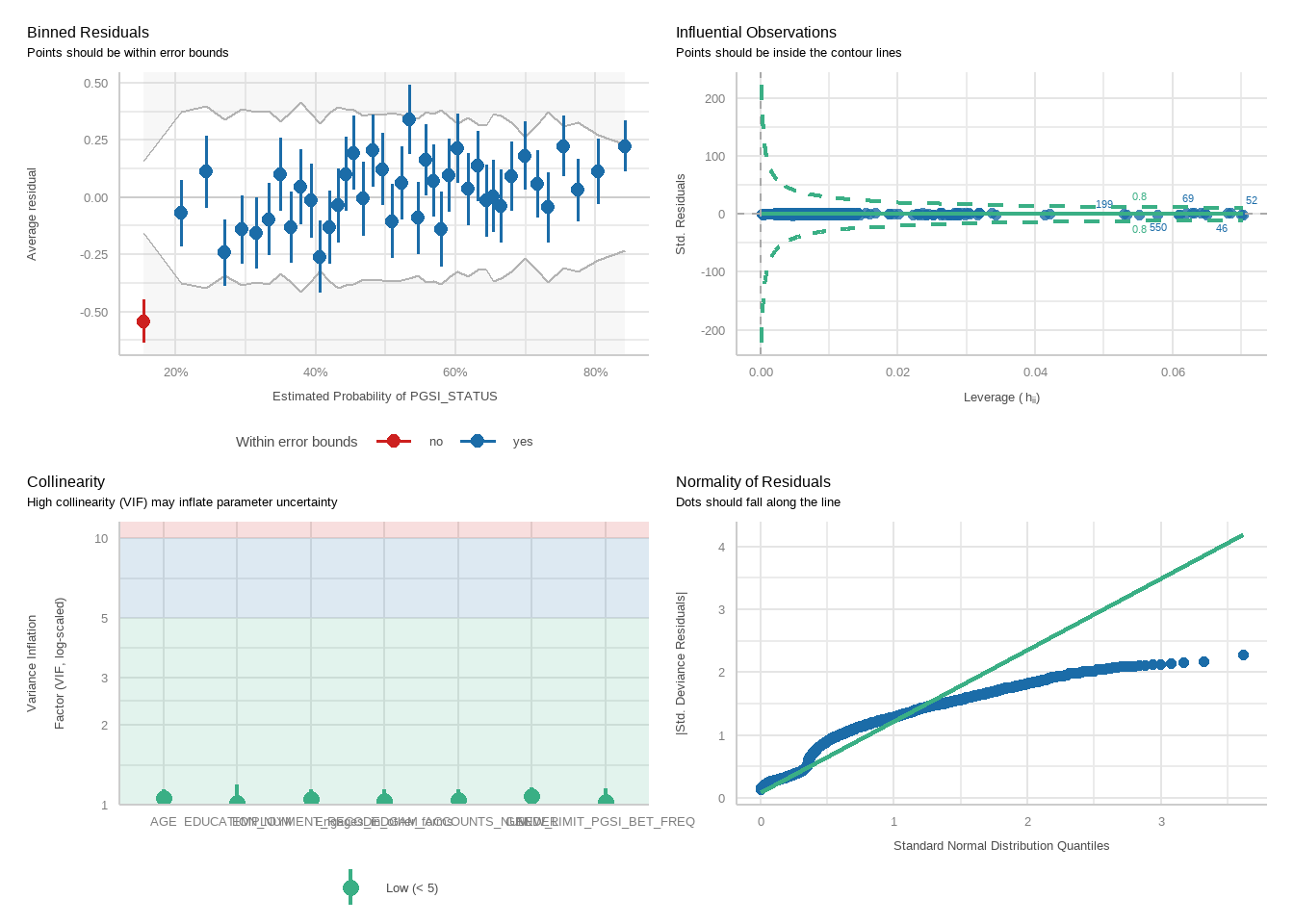
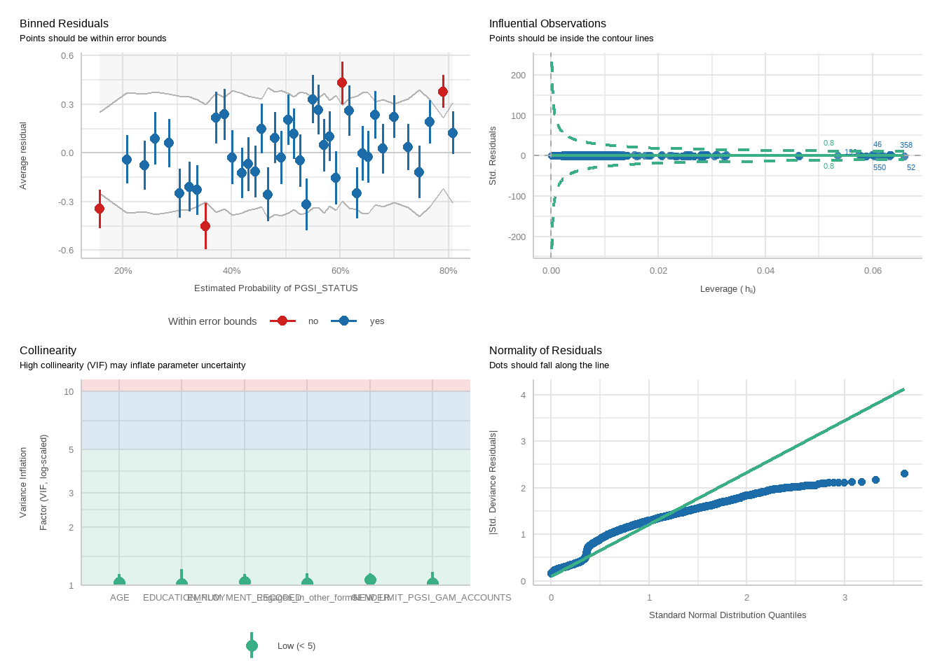
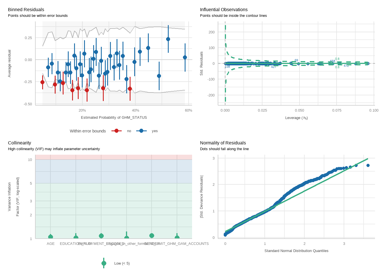
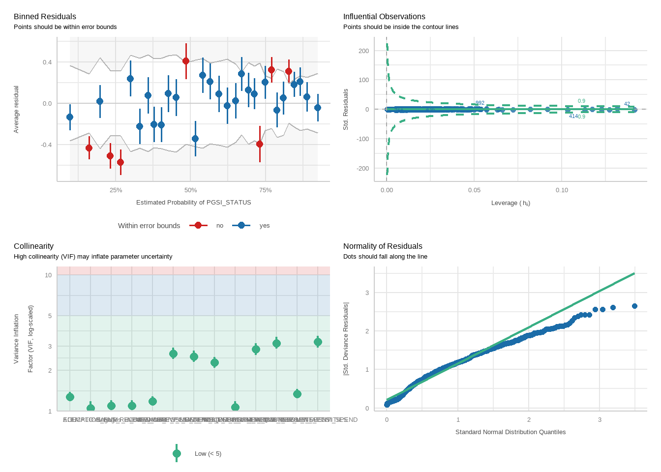
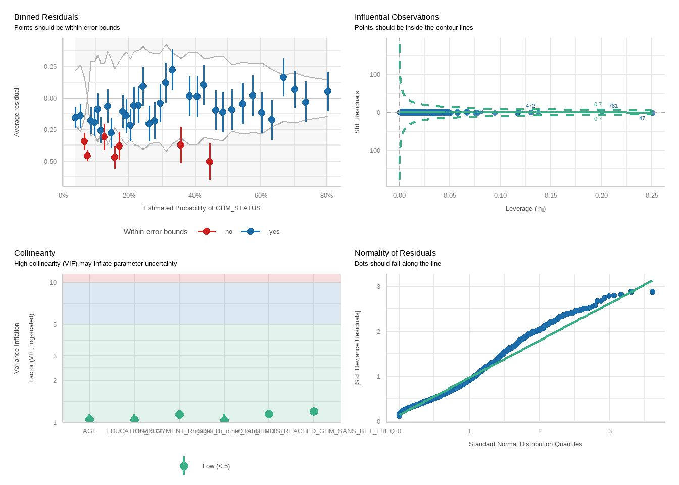
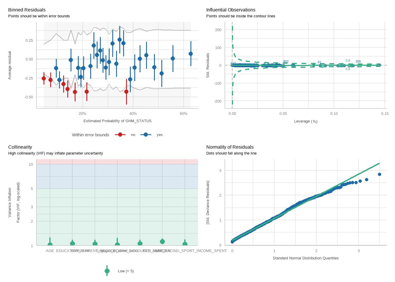
For each model, we will run a function to produce plots showing diagnostic checks and then table regression outcomes together for the PGSI and GHM models, exponentiating betas into odds ratios.
tbl_merge(tbls =list(tbl_weighted_lr_freq_new_limit_PGSI, tbl_weighted_lr_freq_new_limit_GHM),tab_spanner =c("**PGSI Status**", "**GHM Status**")) %>%as_gt() %>%tab_options(data_row.padding =px(1.5)) %>%tab_header(title ="New optimal gambling frequency limit for online wagering as a predictor of harm status (demographic-adjusted models)" )
New optimal gambling frequency limit for online wagering as a predictor of harm status (demographic-adjusted models)
Characteristic
PGSI Status
GHM Status
OR
95% CI
p-value
OR
95% CI
p-value
AGE
0.97
0.96, 0.98
<0.001
0.97
0.96, 0.98
<0.001
GENDER
Female
—
—
—
—
Male
1.74
1.22, 2.49
0.002
2.28
1.36, 3.81
0.002
Unknown
2.24
0.82, 6.12
0.12
2.32
0.71, 7.62
0.2
EMPLOYMENT_RECODED
Employed
—
—
—
—
Unemployed
1.38
0.77, 2.47
0.3
2.72
1.48, 4.99
0.001
Unknown
1.17
0.88, 1.56
0.3
0.98
0.69, 1.40
>0.9
EDUCATION_NUM
0.90
0.83, 0.97
0.007
0.97
0.89, 1.06
0.5
GAM_ACCOUNTS_NUM
1.36
1.23, 1.49
<0.001
1.34
1.20, 1.48
<0.001
Engages_in_other_forms
FALSE
—
—
—
—
TRUE
1.88
1.38, 2.56
<0.001
1.74
1.20, 2.52
0.004
NEW_LIMIT_PGSI_BET_FREQ
1.37
1.07, 1.74
0.012
Null deviance
2,283
1,787
Null df
1,646
1,579
AIC
2,103
1,647
BIC
2,154
1,699
Deviance
2,080
1,625
Residual df
1,637
1,570
No. Obs.
1,647
1,580
NEW_LIMIT_GHM_BET_FREQ
1.37
1.01, 1.85
0.046
Abbreviations: CI = Confidence Interval, OR = Odds Ratio
Calculate Nagelkerke’s R squared for the PGSI model:
# NOTE: R2 is calculate as a proportion here and so in the paper we have multiplied it by 100 to form a percentage value
The model accounts for 15.4854331% of variance in PGSI harm rates.
Calculate Nagelkerke’s R squared for the GHM model:
Show code
NagelkerkeR2_weighted_bet_freq_GHM<-NagelkerkeR2(weighted_lr_freq_new_limit_GHM) %>%as.data.frame() %>%print() # NOTE: R2 is calculate as a proportion here and so in the paper we have multiplied it by 100 to form a percentage value
     N        R2
1 1580 0.1437819
The model accounts for 14.3781926% of variance in PGSI harm rates.
Risk Curve
Let’s plot some risk curves for the relationship between this predictor and the two outcomes. We didn’t pre-register this, but it’s purpose is solely for visual exploration/supplementation and will not be used for inference.
Show code
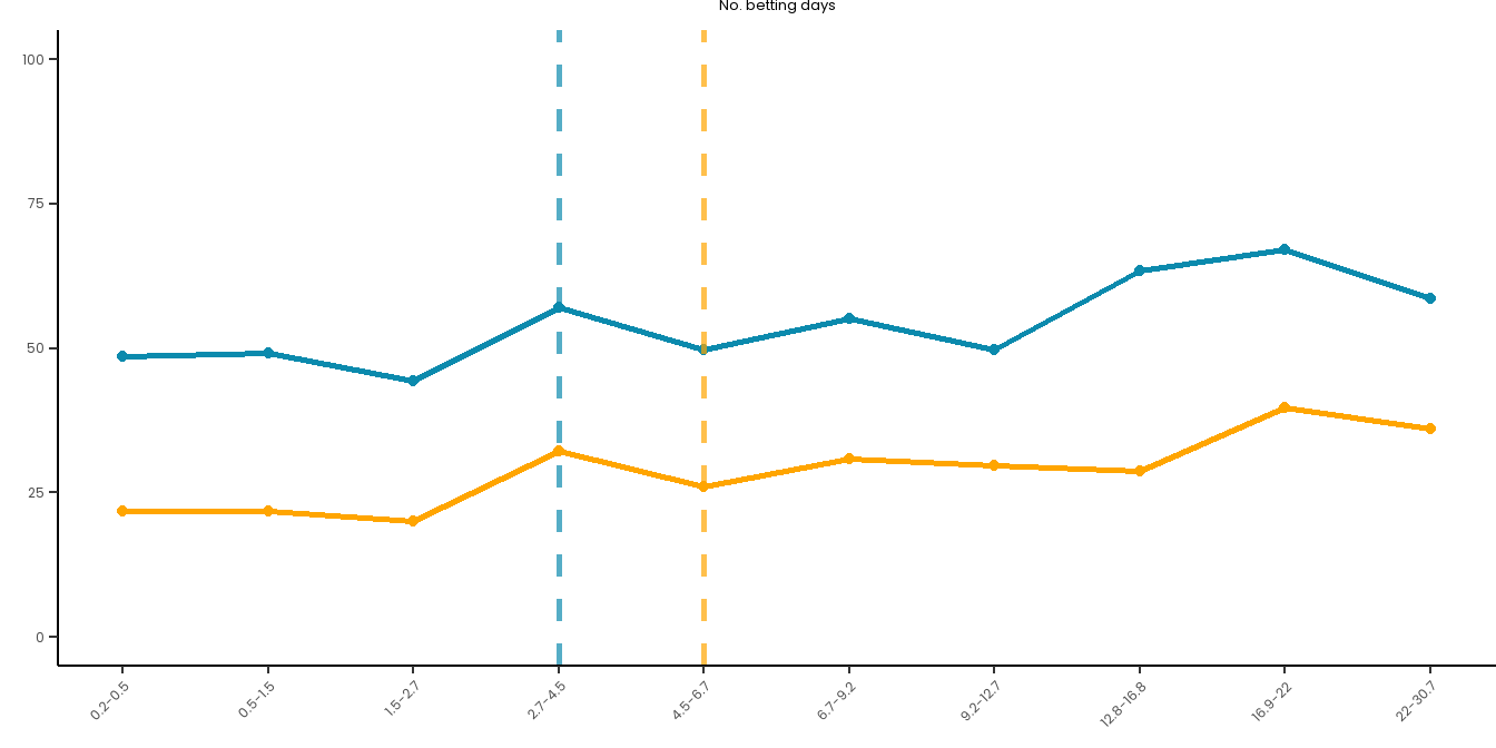
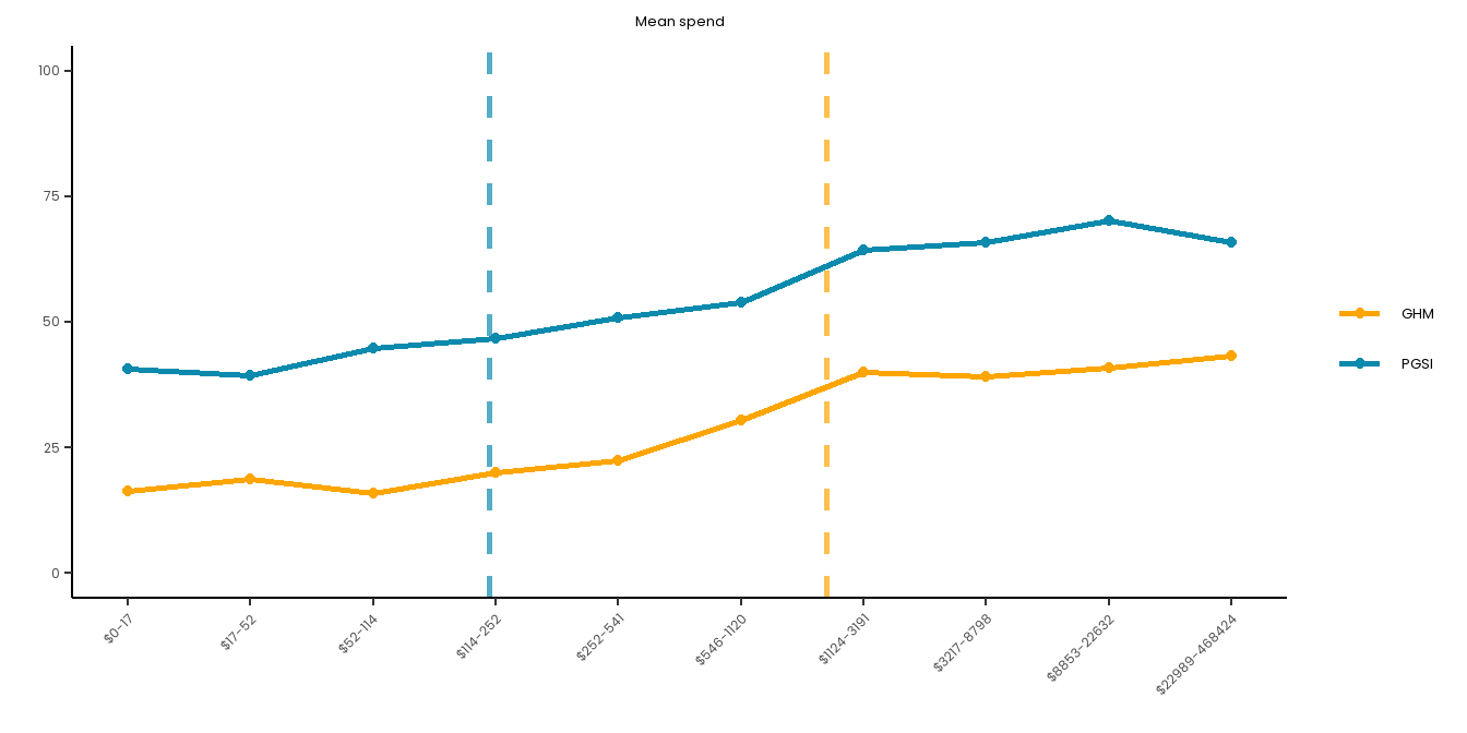
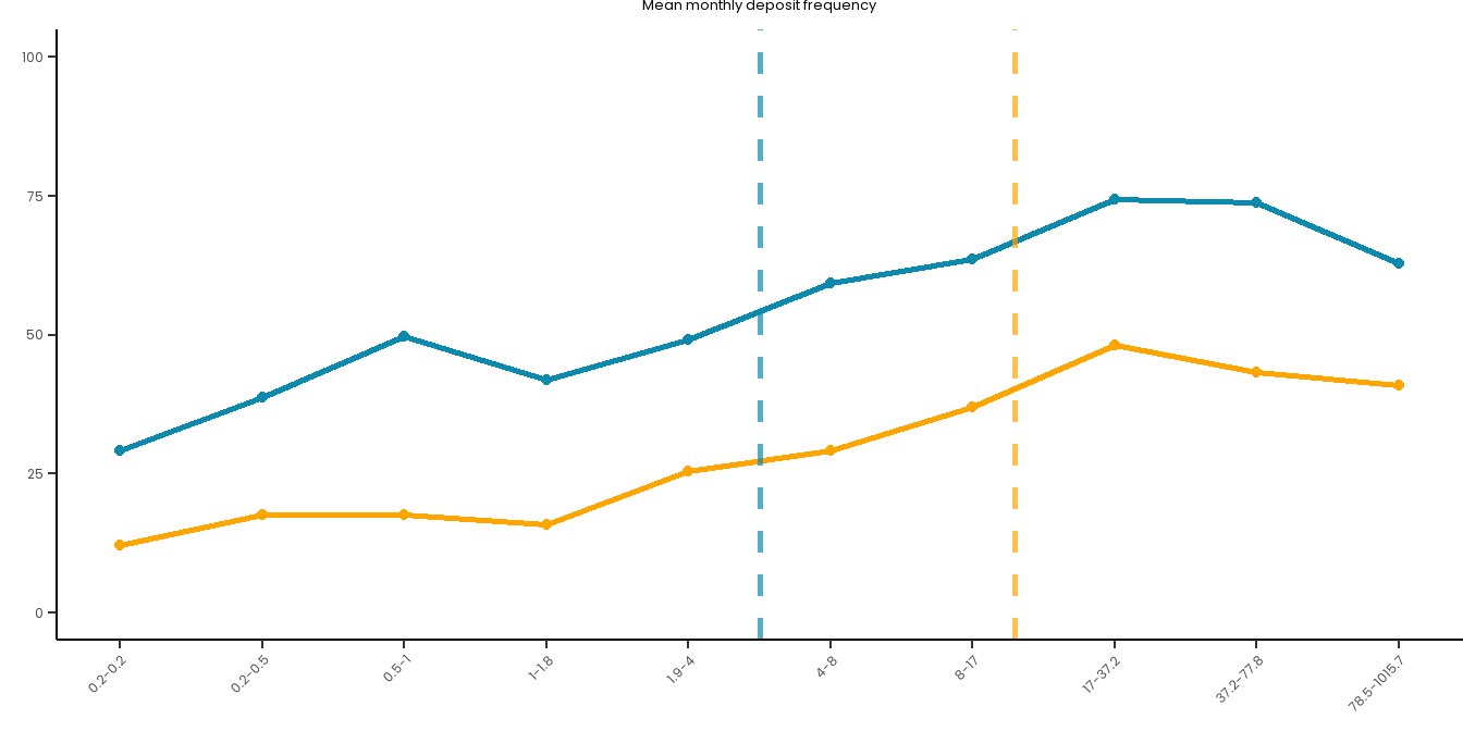
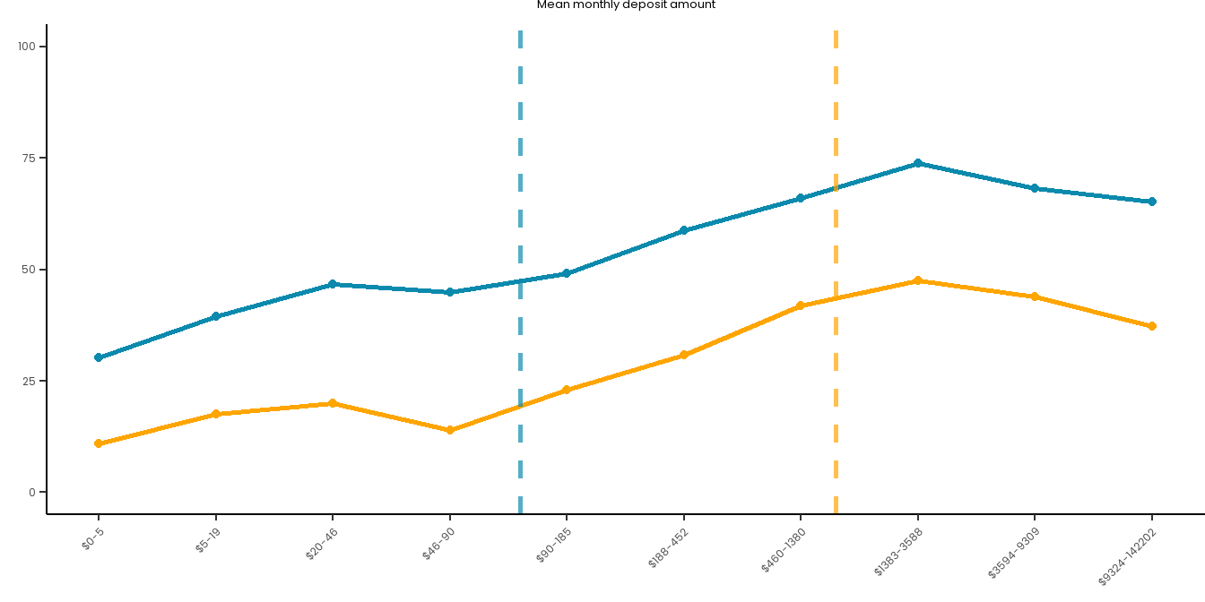
# Set up a good theme for these plots going forward:risk_curve_theme<-theme_classic() +theme(text =element_text(family ="Poppins"),plot.title =element_text(hjust =0.5, size =10, face ="plain"),plot.subtitle =element_text(hjust =0.5, size =13),axis.text.x =element_text(size =9, angle =45, hjust =1),axis.text.y =element_text(size =9),axis.title =element_text(size =10),plot.caption =element_text(size =12),legend.title =element_text(size =12), legend.text =element_text(size =10) ) # Create a summary dataset:summary_data <- master_dataset_recoded_w_new_limits %>%mutate(decile =ntile(PAS_6M_MONTHLY_BET_FREQ_DAYS, 10)) %>%group_by(decile) %>%summarise(PGSI_pct =sum(PGSI_STATUS ==1, na.rm =TRUE) /n() *100,GHM_pct =sum(GHM_STATUS ==1, na.rm =TRUE) /n() *100,min_val =min(PAS_6M_MONTHLY_BET_FREQ_DAYS, na.rm =TRUE),max_val =max(PAS_6M_MONTHLY_BET_FREQ_DAYS, na.rm =TRUE) ) %>%mutate(decile_label =paste(round(min_val, 1), round(max_val, 1), sep ="-"))long_data <- summary_data %>%pivot_longer(cols =c(PGSI_pct, GHM_pct),names_to ="HarmMeasure",values_to ="pct_harmed" ) %>%mutate(HarmMeasure =case_when(HarmMeasure =="PGSI_pct"~"PGSI", HarmMeasure =="GHM_pct"~"GHM"))# Plot both curves on the same plot for ease:combined_risk_curve_betting_freq <-ggplot(long_data, aes(x =as.numeric(decile), y = pct_harmed, color = HarmMeasure, group = HarmMeasure)) +geom_line(size =1) +geom_point() +scale_x_continuous(breaks =1:10, labels = summary_data$decile_label) +labs(title ="No. betting days",x ="",y ="") +ylim(0, 100) +# PGSI LIMIT:geom_vline(xintercept =4, linetype ="dashed", color ="#0B8AAD", size =1, alpha =0.7) +# GHM LIMIT:geom_vline(xintercept =5, linetype ="dashed", color ="orange", size =1, alpha =0.7) +scale_color_manual(name ="", values =c("PGSI"="#0B8AAD", "GHM"="orange")) + risk_curve_theme +theme(legend.position ="none",plot.margin =margin(0,0,-1,0)) combined_risk_curve_betting_freq
# NOTE: R2 is calculate as a proportion here and so in the paper we have multiplied it by 100 to form a percentage value
The model accounts for 17.8140946% of variance in PGSI harm rates.
Calculate Nagelkerke’s R squared for the GHM model:
Show code
NagelkerkeR2_weighted_spend_lr_GHM<-NagelkerkeR2(weighted_lr_spend_new_limit_GHM) %>%as.data.frame() %>%print() # NOTE: R2 is calculate as a proportion here and so in the paper we have multiplied it by 100 to form a percentage value
     N        R2
1 1580 0.1797802
The model accounts for 17.9780248% of variance in PGSI harm rates.
Risk Curve
Plot some risk curves for the relationship between this predictor and the two outcomes.
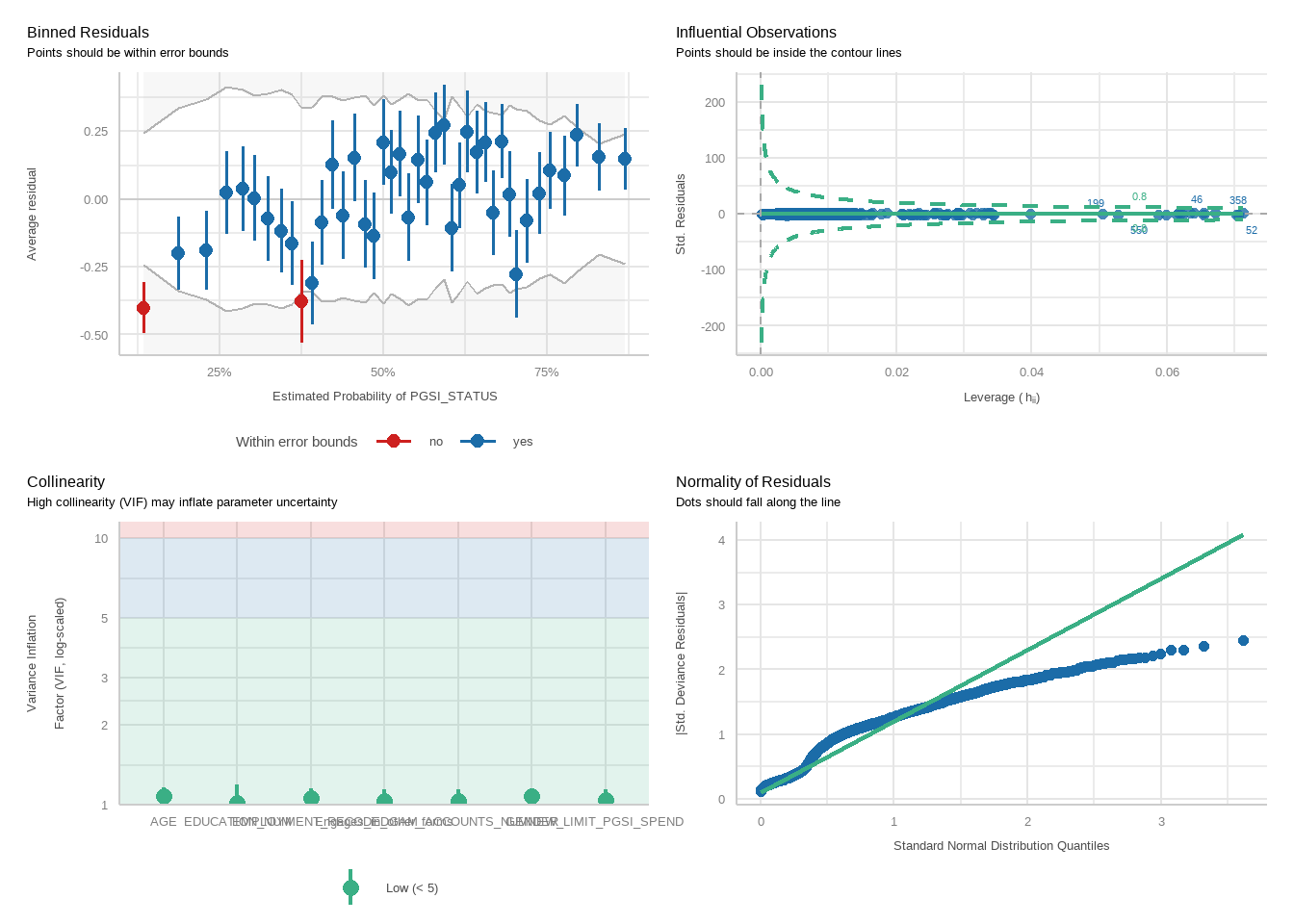
tbl_merge(tbls =list(tbl_weighted_lr_income_spent_new_limit_PGSI, tbl_weighted_lr_income_spent_new_limit_GHM),tab_spanner =c("**PGSI Status**", "**GHM Status**")) %>%as_gt() %>%tab_options(data_row.padding =px(1.5)) %>%tab_header(title ="New optimal percentage of income spent limit for online wagering as a predictor of harm status (demographic-adjusted models)" )
New optimal percentage of income spent limit for online wagering as a predictor of harm status (demographic-adjusted models)
Characteristic
PGSI Status
GHM Status
OR
95% CI
p-value
OR
95% CI
p-value
AGE
0.97
0.96, 0.98
<0.001
0.97
0.96, 0.98
<0.001
GENDER
Female
—
—
—
—
Male
1.73
1.07, 2.80
0.026
2.22
1.16, 4.24
0.015
Unknown
3.82
1.02, 14.3
0.047
1.71
0.44, 6.62
0.4
EMPLOYMENT_RECODED
Employed
—
—
—
—
Unemployed
1.06
0.52, 2.16
0.9
1.58
0.72, 3.46
0.3
EDUCATION_NUM
0.91
0.83, 1.0
0.037
0.99
0.90, 1.09
0.9
GAM_ACCOUNTS_NUM
1.34
1.19, 1.50
<0.001
1.38
1.20, 1.57
<0.001
Engages_in_other_forms
FALSE
—
—
—
—
TRUE
1.93
1.32, 2.82
<0.001
1.97
1.25, 3.10
0.003
NEW_LIMIT_PGSI_INCOME_SPENT
2.83
2.05, 3.93
<0.001
Null deviance
1,527
1,288
Null df
1,054
1,054
AIC
1,362
1,122
BIC
1,404
1,165
Deviance
1,342
1,103
Residual df
1,046
1,046
No. Obs.
1,055
1,055
NEW_LIMIT_GHM_INCOME_SPENT
4.49
3.11, 6.49
<0.001
Abbreviations: CI = Confidence Interval, OR = Odds Ratio
Calculate Nagelkerke’s R squared for the PGSI model:
# NOTE: R2 is calculate as a proportion here and so in the paper we have multiplied it by 100 to form a percentage value
The model accounts for 21.0173697% of variance in PGSI harm rates.
Calculate Nagelkerke’s R squared for the GHM model:
Show code
NagelkerkeR2_weighted_income_spent_lr_GHM<-NagelkerkeR2(weighted_lr_income_spent_new_limit_GHM) %>%as.data.frame() %>%print() # NOTE: R2 is calculate as a proportion here and so in the paper we have multiplied it by 100 to form a percentage value
     N        R2
1 1055 0.2288529
The model accounts for 22.8852894% of variance in PGSI harm rates.
Risk curve
Plot some risk curves for the relationship between this predictor and the two outcomes.
Show code
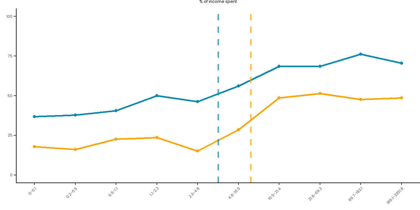
# Create a summary dataset:summary_data <- master_dataset_recoded_w_new_limits %>%mutate(decile =ntile(PERCENT_MON_INCOME_SPENT_MONTHLY_PAS_6M, 10)) %>%group_by(decile) %>%summarise(PGSI_pct =sum(PGSI_STATUS ==1, na.rm =TRUE) /n() *100,GHM_pct =sum(GHM_STATUS ==1, na.rm =TRUE) /n() *100,min_val =min(PERCENT_MON_INCOME_SPENT_MONTHLY_PAS_6M, na.rm =TRUE),max_val =max(PERCENT_MON_INCOME_SPENT_MONTHLY_PAS_6M, na.rm =TRUE) ) %>%mutate(decile_label =paste(round(min_val, 1), round(max_val, 1), sep ="-")) %>%filter(!is.na(decile))long_data <- summary_data %>%pivot_longer(cols =c(PGSI_pct, GHM_pct),names_to ="HarmMeasure",values_to ="pct_harmed" ) %>%mutate(HarmMeasure =case_when(HarmMeasure =="PGSI_pct"~"PGSI", HarmMeasure =="GHM_pct"~"GHM"))# Plot both curves on the same plot for ease:combined_risk_curve_income_spent <-ggplot(long_data, aes(x =as.numeric(decile), y = pct_harmed, color = HarmMeasure, group = HarmMeasure)) +geom_line(size =1) +geom_point() +scale_x_continuous(breaks =1:10, labels = summary_data$decile_label) +labs(title ="% of income spent",x ="",y ="") +ylim(0, 100) +# PGSI LIMIT:geom_vline(xintercept =5.5, linetype ="dashed", color ="#0B8AAD", size =1, alpha =0.7) +# GHM LIMIT:geom_vline(xintercept =6.3, linetype ="dashed", color ="orange", size =1, alpha =0.7) +scale_color_manual(name ="", values =c("PGSI"="#0B8AAD", "GHM"="orange")) + risk_curve_theme +theme(legend.position ="none",plot.margin =margin(0,0,-1,0)) combined_risk_curve_income_spent
tbl_merge(tbls =list(tbl_weighted_lr_n_activities_new_limit_PGSI, tbl_weighted_lr_n_activities_new_limit_GHM),tab_spanner =c("**PGSI Status**", "**GHM Status**")) %>%as_gt() %>%tab_options(data_row.padding =px(1.5)) %>%tab_header(title ="New optimal number of different sport and race types limit for online wagering as a predictor of harm status (demographic-adjusted models)" )
New optimal number of different sport and race types limit for online wagering as a predictor of harm status (demographic-adjusted models)
Characteristic
PGSI Status
GHM Status
OR
95% CI
p-value
OR
95% CI
p-value
AGE
0.97
0.97, 0.98
<0.001
0.97
0.96, 0.98
<0.001
GENDER
Female
—
—
—
—
Male
1.68
1.17, 2.40
0.005
2.25
1.34, 3.78
0.002
Unknown
2.19
0.84, 5.70
0.11
2.36
0.73, 7.64
0.2
EMPLOYMENT_RECODED
Employed
—
—
—
—
Unemployed
1.40
0.78, 2.51
0.3
2.80
1.51, 5.18
0.001
Unknown
1.16
0.87, 1.55
0.3
0.99
0.70, 1.41
>0.9
EDUCATION_NUM
0.90
0.83, 0.97
0.007
0.97
0.89, 1.06
0.5
GAM_ACCOUNTS_NUM
1.34
1.22, 1.48
<0.001
1.33
1.19, 1.47
<0.001
Engages_in_other_forms
FALSE
—
—
—
—
TRUE
1.92
1.40, 2.63
<0.001
1.78
1.22, 2.60
0.003
NEW_LIMIT_PGSI_N_ACTIVITIES
1.55
1.20, 2.00
<0.001
Null deviance
2,283
1,787
Null df
1,646
1,579
AIC
2,096
1,649
BIC
2,147
1,700
Deviance
2,073
1,626
Residual df
1,637
1,570
No. Obs.
1,647
1,580
NEW_LIMIT_GHM_N_ACTIVITIES
1.30
0.95, 1.77
0.10
Abbreviations: CI = Confidence Interval, OR = Odds Ratio
Calculate Nagelkerke’s R squared for the PGSI model:
# NOTE: R2 is calculate as a proportion here and so in the paper we have multiplied it by 100 to form a percentage value
The model accounts for 15.9464454% of variance in PGSI harm rates.
Calculate Nagelkerke’s R squared for the GHM model:
Show code
NagelkerkeR2_weighted_n_activities_lr_GHM<-NagelkerkeR2(weighted_lr_n_activities_new_limit_GHM) %>%as.data.frame() %>%print() # NOTE: R2 is calculate as a proportion here and so in the paper we have multiplied it by 100 to form a percentage value
     N        R2
1 1580 0.1425208
The model accounts for 14.2520775% of variance in PGSI harm rates.
Risk Curve
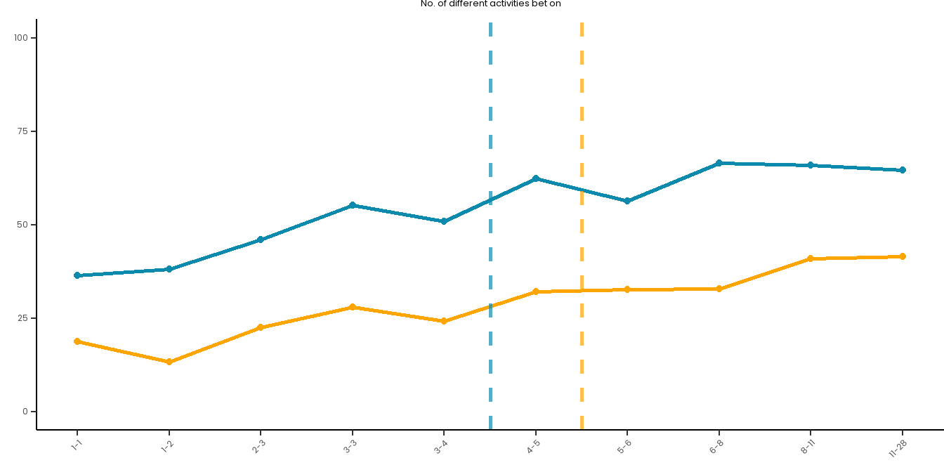
Plot some risk curves for the relationship between this predictor and the two outcomes.
Show code
# Create a summary dataset:summary_data <- master_dataset_recoded_w_new_limits %>%mutate(decile =ntile(PAS_6M_N_ACTIVITIES, 10)) %>%group_by(decile) %>%summarise(PGSI_pct =sum(PGSI_STATUS ==1, na.rm =TRUE) /n() *100,GHM_pct =sum(GHM_STATUS ==1, na.rm =TRUE) /n() *100,min_val =min(PAS_6M_N_ACTIVITIES, na.rm =TRUE),max_val =max(PAS_6M_N_ACTIVITIES, na.rm =TRUE) ) %>%mutate(decile_label =paste(round(min_val, 2), round(max_val, 2), sep ="-")) %>%filter(!is.na(decile))long_data <- summary_data %>%pivot_longer(cols =c(PGSI_pct, GHM_pct),names_to ="HarmMeasure",values_to ="pct_harmed" ) %>%mutate(HarmMeasure =case_when(HarmMeasure =="PGSI_pct"~"PGSI", HarmMeasure =="GHM_pct"~"GHM"))# Plot both curves on the same plot for ease:combined_risk_curve_n_activities <-ggplot(long_data, aes(x =as.numeric(decile), y = pct_harmed, color = HarmMeasure, group = HarmMeasure)) +geom_line(size =1) +geom_point() +scale_x_continuous(breaks =1:10, labels = summary_data$decile_label) +labs(title ="No. of different activities bet on",x ="",y ="") +ylim(0, 100) +# PGSI LIMIT:geom_vline(xintercept =5.5, linetype ="dashed", color ="#0B8AAD", size =1, alpha =0.7) +# GHM LIMIT:geom_vline(xintercept =6.5, linetype ="dashed", color ="orange", size =1, alpha =0.7) +scale_color_manual(name ="", values =c("PGSI"="#0B8AAD", "GHM"="orange")) + risk_curve_theme +theme(legend.position ="none",plot.margin =margin(0,0,-1,0)) combined_risk_curve_n_activities
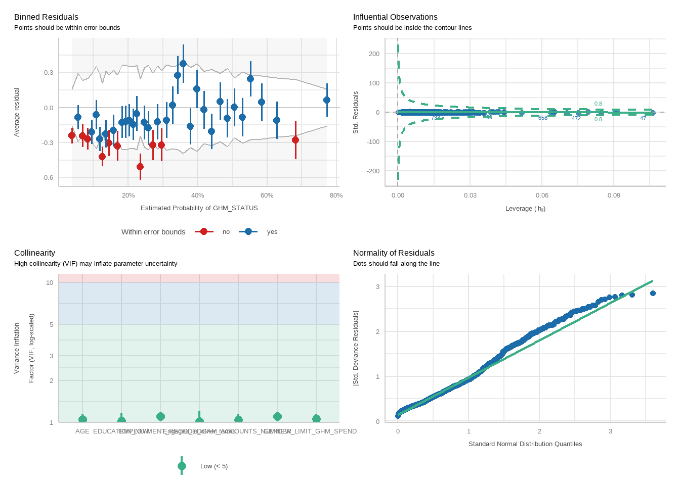
tbl_merge(tbls =list(tbl_weighted_lr_deposit_freq_new_limit_PGSI, tbl_weighted_lr_deposit_freq_new_limit_GHM),tab_spanner =c("**PGSI Status**", "**GHM Status**")) %>%as_gt() %>%tab_options(data_row.padding =px(1.5)) %>%tab_header(title ="New optimal deposit frequency limit for online wagering as a predictor of harm status (demographic-adjusted models)" )
New optimal deposit frequency limit for online wagering as a predictor of harm status (demographic-adjusted models)
Characteristic
PGSI Status
GHM Status
OR
95% CI
p-value
OR
95% CI
p-value
AGE
0.97
0.97, 0.98
<0.001
0.97
0.96, 0.98
<0.001
GENDER
Female
—
—
—
—
Male
1.60
1.11, 2.29
0.011
2.12
1.27, 3.54
0.004
Unknown
2.02
0.72, 5.67
0.2
1.74
0.49, 6.19
0.4
EMPLOYMENT_RECODED
Employed
—
—
—
—
Unemployed
1.38
0.76, 2.50
0.3
2.63
1.45, 4.79
0.002
Unknown
1.06
0.79, 1.43
0.7
0.90
0.62, 1.31
0.6
EDUCATION_NUM
0.91
0.84, 0.98
0.015
0.98
0.89, 1.07
0.6
GAM_ACCOUNTS_NUM
1.36
1.24, 1.50
<0.001
1.37
1.23, 1.53
<0.001
Engages_in_other_forms
FALSE
—
—
—
—
TRUE
1.94
1.41, 2.66
<0.001
1.75
1.19, 2.56
0.004
NEW_LIMIT_PGSI_DEPOSIT_FREQ
2.60
2.01, 3.36
<0.001
Null deviance
2,283
1,787
Null df
1,646
1,579
AIC
2,041
1,590
BIC
2,091
1,641
Deviance
2,017
1,567
Residual df
1,637
1,570
No. Obs.
1,647
1,580
NEW_LIMIT_GHM_DEPOSIT_FREQ
3.39
2.42, 4.75
<0.001
Abbreviations: CI = Confidence Interval, OR = Odds Ratio
Calculate Nagelkerke’s R squared for the PGSI model:
# NOTE: R2 is calculate as a proportion here and so in the paper we have multiplied it by 100 to form a percentage value
The model accounts for 19.8684028% of variance in PGSI harm rates.
Calculate Nagelkerke’s R squared for the GHM model:
Show code
NagelkerkeR2_weighted_deposit_freq_lr_GHM<-NagelkerkeR2(weighted_lr_deposit_freq_new_limit_GHM) %>%as.data.frame() %>%print() # NOTE: R2 is calculate as a proportion here and so in the paper we have multiplied it by 100 to form a percentage value
     N        R2
1 1580 0.1915685
The model accounts for 19.1568532% of variance in PGSI harm rates.
Risk Curve
Plot some risk curves for the relationship between this predictor and the two outcomes.
# NOTE: R2 is calculate as a proportion here and so in the paper we have multiplied it by 100 to form a percentage value
The model accounts for 19.0144593% of variance in PGSI harm rates.
Calculate Nagelkerke’s R squared for the GHM model:
Show code
NagelkerkeR2_weighted_deposit_amount_lr_GHM<-NagelkerkeR2(weighted_lr_deposit_amount_new_limit_GHM) %>%as.data.frame() %>%print() # NOTE: R2 is calculate as a proportion here and so in the paper we have multiplied it by 100 to form a percentage value
     N        R2
1 1580 0.1824433
The model accounts for 18.2443336% of variance in PGSI harm rates.
Risk curve
Plot some risk curves for the relationship between this predictor and the two outcomes.
tbl_merge(tbls =list(tbl_weighted_lr_income_deposited_new_limit_PGSI, tbl_weighted_lr_income_deposited_new_limit_GHM),tab_spanner =c("**PGSI Status**", "**GHM Status**")) %>%as_gt() %>%tab_options(data_row.padding =px(1.5)) %>%tab_header(title ="New optimal amount of income deposited limit for online wagering as a predictor of harm status (demographic-adjusted models)" )
New optimal amount of income deposited limit for online wagering as a predictor of harm status (demographic-adjusted models)
Characteristic
PGSI Status
GHM Status
OR
95% CI
p-value
OR
95% CI
p-value
AGE
0.97
0.96, 0.98
<0.001
0.97
0.96, 0.98
<0.001
GENDER
Female
—
—
—
—
Male
1.71
1.06, 2.76
0.028
2.53
1.28, 4.97
0.007
Unknown
3.53
0.92, 13.6
0.067
2.09
0.32, 13.8
0.4
EMPLOYMENT_RECODED
Employed
—
—
—
—
Unemployed
1.06
0.52, 2.17
0.9
1.92
0.84, 4.38
0.12
EDUCATION_NUM
0.91
0.84, 1.00
0.045
0.96
0.87, 1.06
0.4
GAM_ACCOUNTS_NUM
1.35
1.20, 1.52
<0.001
1.40
1.23, 1.60
<0.001
Engages_in_other_forms
FALSE
—
—
—
—
TRUE
2.15
1.44, 3.19
<0.001
1.96
1.20, 3.18
0.007
NEW_LIMIT_PGSI_INCOME_DEPOSITED
3.78
2.70, 5.30
<0.001
Null deviance
1,527
1,288
Null df
1,054
1,054
AIC
1,330
1,122
BIC
1,373
1,164
Deviance
1,310
1,101
Residual df
1,046
1,046
No. Obs.
1,055
1,055
NEW_LIMIT_GHM_INCOME_DEPOSITED
7.10
4.50, 11.2
<0.001
Abbreviations: CI = Confidence Interval, OR = Odds Ratio
Calculate Nagelkerke’s R squared for the PGSI model:
# NOTE: R2 is calculate as a proportion here and so in the paper we have multiplied it by 100 to form a percentage value
The model accounts for 24.2618149% of variance in PGSI harm rates.
Calculate Nagelkerke’s R squared for the GHM model:
Show code
NagelkerkeR2_weighted_income_deposited_lr_GHM<-NagelkerkeR2(weighted_lr_income_deposited_new_limit_GHM) %>%as.data.frame() %>%print() # NOTE: R2 is calculate as a proportion here and so in the paper we have multiplied it by 100 to form a percentage value
     N        R2
1 1055 0.2307804
The model accounts for 23.0780376% of variance in PGSI harm rates.
Risk curve
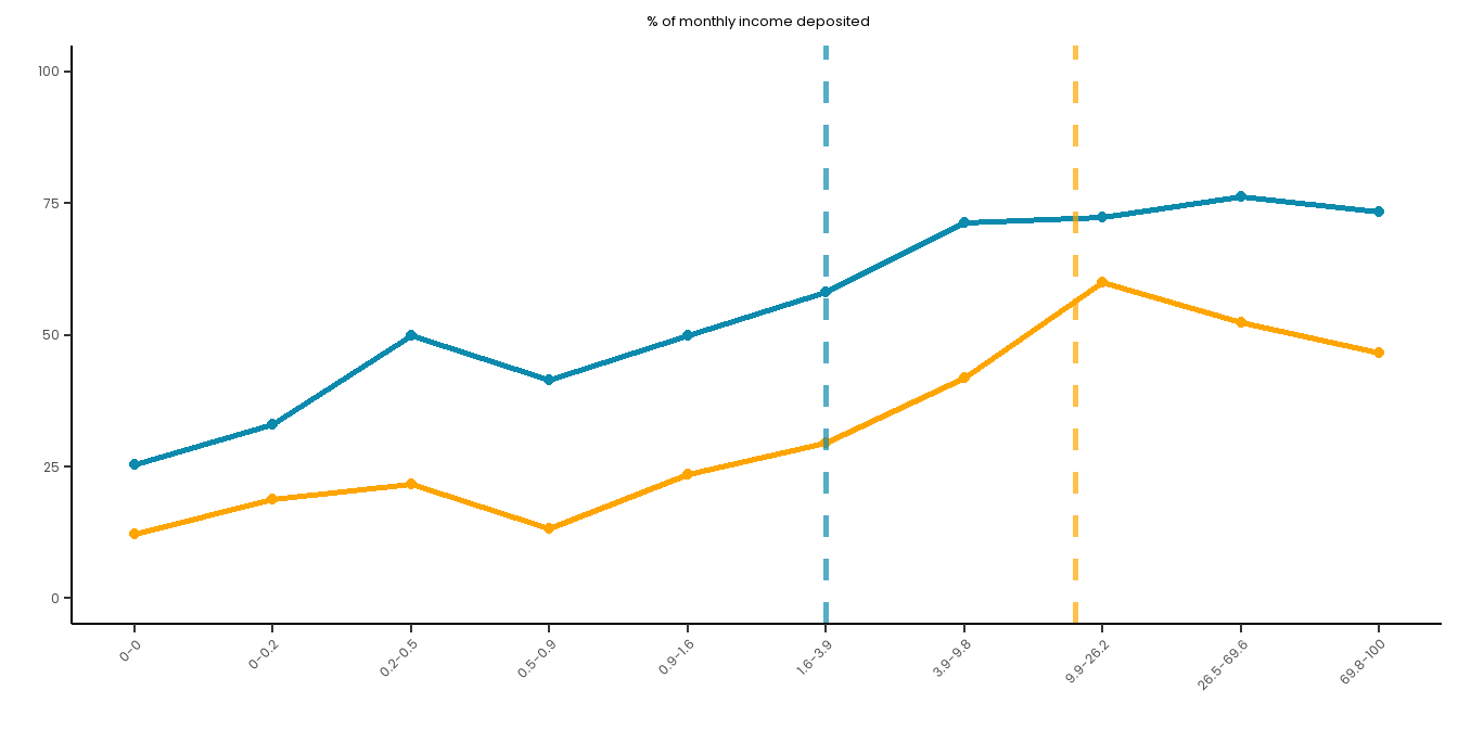
Plot some risk curves for the relationship between this predictor and the two outcomes.
Show code
# Create a summary dataset:summary_data <- master_dataset_recoded_w_new_limits %>%mutate(decile =ntile(PERCENT_MON_INCOME_DEPOSIT_MONTHLY_PAS_6M, 10)) %>%group_by(decile) %>%summarise(PGSI_pct =sum(PGSI_STATUS ==1, na.rm =TRUE) /n() *100,GHM_pct =sum(GHM_STATUS ==1, na.rm =TRUE) /n() *100,min_val =min(PERCENT_MON_INCOME_DEPOSIT_MONTHLY_PAS_6M, na.rm =TRUE),max_val =max(PERCENT_MON_INCOME_DEPOSIT_MONTHLY_PAS_6M, na.rm =TRUE) ) %>%mutate(decile_label =paste(round(min_val, 1), round(max_val, 1), sep ="-")) %>%filter(!is.na(decile))long_data <- summary_data %>%pivot_longer(cols =c(PGSI_pct, GHM_pct),names_to ="HarmMeasure",values_to ="pct_harmed" ) %>%mutate(HarmMeasure =case_when(HarmMeasure =="PGSI_pct"~"PGSI", HarmMeasure =="GHM_pct"~"GHM"))# Plot both curves on the same plot for ease:combined_risk_curve_income_deposited<-ggplot(long_data, aes(x =as.numeric(decile), y = pct_harmed, color = HarmMeasure, group = HarmMeasure)) +geom_line(size =1) +geom_point() +scale_x_continuous(breaks =1:10, labels = summary_data$decile_label) +labs(title ="% of monthly income deposited",x ="",y ="") +ylim(0, 100) + risk_curve_theme +# PGSI LIMIT:geom_vline(xintercept =6, linetype ="dashed", color ="#0B8AAD", size =1, alpha =0.7) +# GHM LIMIT:geom_vline(xintercept =7.8, linetype ="dashed", color ="orange", size =1, alpha =0.7) +scale_color_manual(name ="", values =c("PGSI"="#0B8AAD", "GHM"="orange")) +theme(legend.position ="none")combined_risk_curve_income_deposited
tbl_merge(tbls =list(tbl_weighted_lr_gam_accounts_new_limit_PGSI, tbl_weighted_lr_gam_accounts_new_limit_GHM),tab_spanner =c("**PGSI Status**", "**GHM Status**")) %>%as_gt() %>%tab_options(data_row.padding =px(1.5)) %>%tab_header(title ="New optimal number of wagering accounts limit for online wagering as a predictor of harm status (demographic-adjusted models)" )
New optimal number of wagering accounts limit for online wagering as a predictor of harm status (demographic-adjusted models)
Characteristic
PGSI Status
GHM Status
OR
95% CI
p-value
OR
95% CI
p-value
AGE
0.97
0.96, 0.98
<0.001
0.97
0.96, 0.98
<0.001
GENDER
Female
—
—
—
—
Male
1.82
1.27, 2.61
0.001
2.62
1.57, 4.38
<0.001
Unknown
2.51
0.98, 6.39
0.054
2.96
0.91, 9.57
0.070
EMPLOYMENT_RECODED
Employed
—
—
—
—
Unemployed
1.36
0.77, 2.39
0.3
2.74
1.49, 5.05
0.001
Unknown
1.16
0.87, 1.54
0.3
0.96
0.68, 1.36
0.8
EDUCATION_NUM
0.90
0.83, 0.97
0.007
0.97
0.89, 1.06
0.5
Engages_in_other_forms
FALSE
—
—
—
—
TRUE
1.88
1.38, 2.57
<0.001
1.77
1.22, 2.57
0.003
NEW_LIMIT_PGSI_GAM_ACCOUNTS
2.17
1.71, 2.76
<0.001
Null deviance
2,283
1,787
Null df
1,646
1,579
AIC
2,108
1,665
BIC
2,154
1,711
Deviance
2,087
1,645
Residual df
1,638
1,571
No. Obs.
1,647
1,580
NEW_LIMIT_GHM_GAM_ACCOUNTS
1.83
1.38, 2.44
<0.001
Abbreviations: CI = Confidence Interval, OR = Odds Ratio
Calculate Nagelkerke’s R squared for the PGSI model:
# NOTE: R2 is calculate as a proportion here and so in the paper we have multiplied it by 100 to form a percentage value
The model accounts for 14.9389916% of variance in PGSI harm rates.
Calculate Nagelkerke’s R squared for the GHM model:
Show code
NagelkerkeR2_weighted_gam_accounts_lr_GHM<-NagelkerkeR2(weighted_lr_gam_accounts_new_limit_GHM) %>%as.data.frame() %>%print() # NOTE: R2 is calculate as a proportion here and so in the paper we have multiplied it by 100 to form a percentage value
     N        R2
1 1580 0.1266771
The model accounts for 12.6677066% of variance in PGSI harm rates.
Risk curve
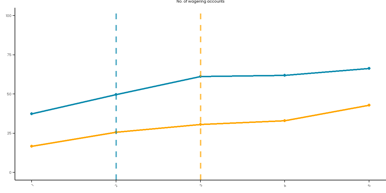
Plot some risk curves for the relationship between this predictor and the two outcomes. We won’t use deciles here as the values are so low in range:
Show code
# Create a summary dataset:summary_data <- master_dataset_recoded_w_new_limits %>%group_by(GAM_ACCOUNTS_NUM) %>%summarise(PGSI_pct =sum(PGSI_STATUS ==1, na.rm =TRUE) /n() *100,GHM_pct =sum(GHM_STATUS ==1, na.rm =TRUE) /n() *100 ) long_data <- summary_data %>%pivot_longer(cols =c(PGSI_pct, GHM_pct),names_to ="HarmMeasure",values_to ="pct_harmed" ) %>%mutate(HarmMeasure =case_when(HarmMeasure =="PGSI_pct"~"PGSI", HarmMeasure =="GHM_pct"~"GHM"))# Plot both curves on the same plot for ease:combined_risk_curve_n_accounts<-ggplot(long_data, aes(x = GAM_ACCOUNTS_NUM, y = pct_harmed,color = HarmMeasure, group = HarmMeasure)) +geom_line(size =1) +geom_point() +ylim(0, 100) +scale_x_continuous(breaks =1:5) +labs(title ="No. of wagering accounts", x ="",y ="") +# PGSI LIMIT:geom_vline(xintercept =2, linetype ="dashed", color ="#0B8AAD", size =1, alpha =0.7) +# GHM LIMIT:geom_vline(xintercept =3, linetype ="dashed", color ="orange", size =1, alpha =0.7) +scale_color_manual(name ="", values =c("PGSI"="#0B8AAD", "GHM"="orange")) + risk_curve_theme +theme(legend.position ="none",plot.margin =margin(0,0,-1,0)) combined_risk_curve_n_accounts
All-limit adjusted model
And now perform the models that incorporate all of the new limits to determine the independent predictive ability of each limit:
tbl_merge(tbls =list(tbl_weighted_lr_all_limit_PGSI, tbl_weighted_lr_all_limit_GHM),tab_spanner =c("**PGSI Status**", "**GHM Status**")) %>%as_gt() %>%tab_options(data_row.padding =px(1.5)) %>%tab_header(title ="New optimal limits for online wagering as a predictor of harm status (demographic- and limit-adjusted models)" )
New optimal limits for online wagering as a predictor of harm status (demographic- and limit-adjusted models)
Characteristic
PGSI Status
GHM Status
OR
95% CI
p-value
OR
95% CI
p-value
AGE
0.98
0.96, 0.99
<0.001
0.97
0.96, 0.99
<0.001
GENDER
Female
—
—
—
—
Male
1.65
1.01, 2.71
0.047
2.64
1.32, 5.26
0.006
Unknown
3.01
0.83, 10.9
0.094
2.18
0.45, 10.7
0.3
EMPLOYMENT_RECODED
Employed
—
—
—
—
Unemployed
1.16
0.55, 2.43
0.7
1.58
0.72, 3.44
0.3
EDUCATION_NUM
0.93
0.85, 1.02
0.12
0.99
0.90, 1.10
>0.9
Engages_in_other_forms
FALSE
—
—
—
—
TRUE
2.22
1.46, 3.36
<0.001
2.11
1.29, 3.45
0.003
NEW_LIMIT_PGSI_BET_FREQ
0.36
0.22, 0.60
<0.001
NEW_LIMIT_PGSI_SPEND
1.18
0.68, 2.04
0.6
NEW_LIMIT_PGSI_INCOME_SPENT
1.23
0.68, 2.22
0.5
NEW_LIMIT_PGSI_N_ACTIVITIES
1.25
0.87, 1.81
0.2
NEW_LIMIT_PGSI_DEPOSIT_FREQ
2.25
1.36, 3.73
0.002
NEW_LIMIT_PGSI_DEPOSIT_AMOUNT
1.48
0.91, 2.40
0.12
NEW_LIMIT_PGSI_INCOME_DEPOSITED
2.21
1.25, 3.90
0.007
NEW_LIMIT_PGSI_GAM_ACCOUNTS
1.94
1.41, 2.65
<0.001
Null deviance
1,527
1,288
Null df
1,054
1,054
AIC
1,311
1,100
BIC
1,379
1,168
Deviance
1,274
1,063
Residual df
1,040
1,040
No. Obs.
1,055
1,055
NEW_LIMIT_GHM_BET_FREQ
0.27
0.14, 0.51
<0.001
NEW_LIMIT_GHM_SPEND
1.31
0.57, 3.01
0.5
NEW_LIMIT_GHM_INCOME_SPENT
3.50
1.94, 6.34
<0.001
NEW_LIMIT_GHM_N_ACTIVITIES
0.92
0.59, 1.43
0.7
NEW_LIMIT_GHM_DEPOSIT_FREQ
3.12
1.63, 5.98
<0.001
NEW_LIMIT_GHM_DEPOSIT_AMOUNT
0.63
0.25, 1.55
0.3
NEW_LIMIT_GHM_INCOME_DEPOSITED
3.22
1.48, 6.98
0.003
NEW_LIMIT_GHM_GAM_ACCOUNTS
2.04
1.42, 2.95
<0.001
Abbreviations: CI = Confidence Interval, OR = Odds Ratio
Calculate Nagelkerke’s R squared for the PGSI model:
# NOTE: R2 is calculate as a proportion here and so in the paper we have multiplied it by 100 to form a percentage value
The model accounts for 27.8025472% of variance in PGSI harm rates.
Calculate Nagelkerke’s R squared for the GHM model:
Show code
NagelkerkeR2_weighted_all_limit_lr_GHM<-NagelkerkeR2(weighted_lr_all_limit_GHM) %>%as.data.frame() %>%print() # NOTE: R2 is calculate as a proportion here and so in the paper we have multiplied it by 100 to form a percentage value
     N        R2
1 1055 0.2724964
The model accounts for 27.2496388% of variance in PGSI harm rates.
Show code
# First, extract the model coefficients:model_coefs <-coef(weighted_lr_all_limit_PGSI)# Define the NEW_LIMIT variables in the order you want to accumulate them.# (Change the order below if you wish to follow a different sequence.)new_limit_vars <-c( "NEW_LIMIT_PGSI_DEPOSIT_FREQ","NEW_LIMIT_PGSI_INCOME_DEPOSITED","NEW_LIMIT_PGSI_GAM_ACCOUNTS")# Extract the intercept (baseline for a reference person, with demographics at reference)baseline <- model_coefs["(Intercept)"]# Initialize a vector to store the cumulative linear predictors (z)cumulative_z <-numeric(length(new_limit_vars))# And a vector to store probabilitiescumulative_prob <-numeric(length(new_limit_vars))# Loop through the NEW_LIMIT variables in the specified orderfor(i inseq_along(new_limit_vars)) {# For the cumulative effect, add the coefficient for the current indicator.# For the first indicator, add it to the intercept;# for subsequent ones, add the new coefficient to the previous cumulative sum.if(i ==1) { cumulative_z[i] <- baseline + model_coefs[new_limit_vars[i]] } else { cumulative_z[i] <- cumulative_z[i -1] + model_coefs[new_limit_vars[i]] }# Compute the predicted probability using the logistic function: cumulative_prob[i] <-exp(cumulative_z[i]) / (1+exp(cumulative_z[i]))}# Create a summary table:cumulative_summary <-data.frame("Number_of_Indicators"=1:length(new_limit_vars),"Cumulative_z"=round(cumulative_z, 3),"Predicted_Probability"=round(cumulative_prob, 3),"Predicted_Probability_Percent"=round(cumulative_prob *100, 1))print(cumulative_summary)
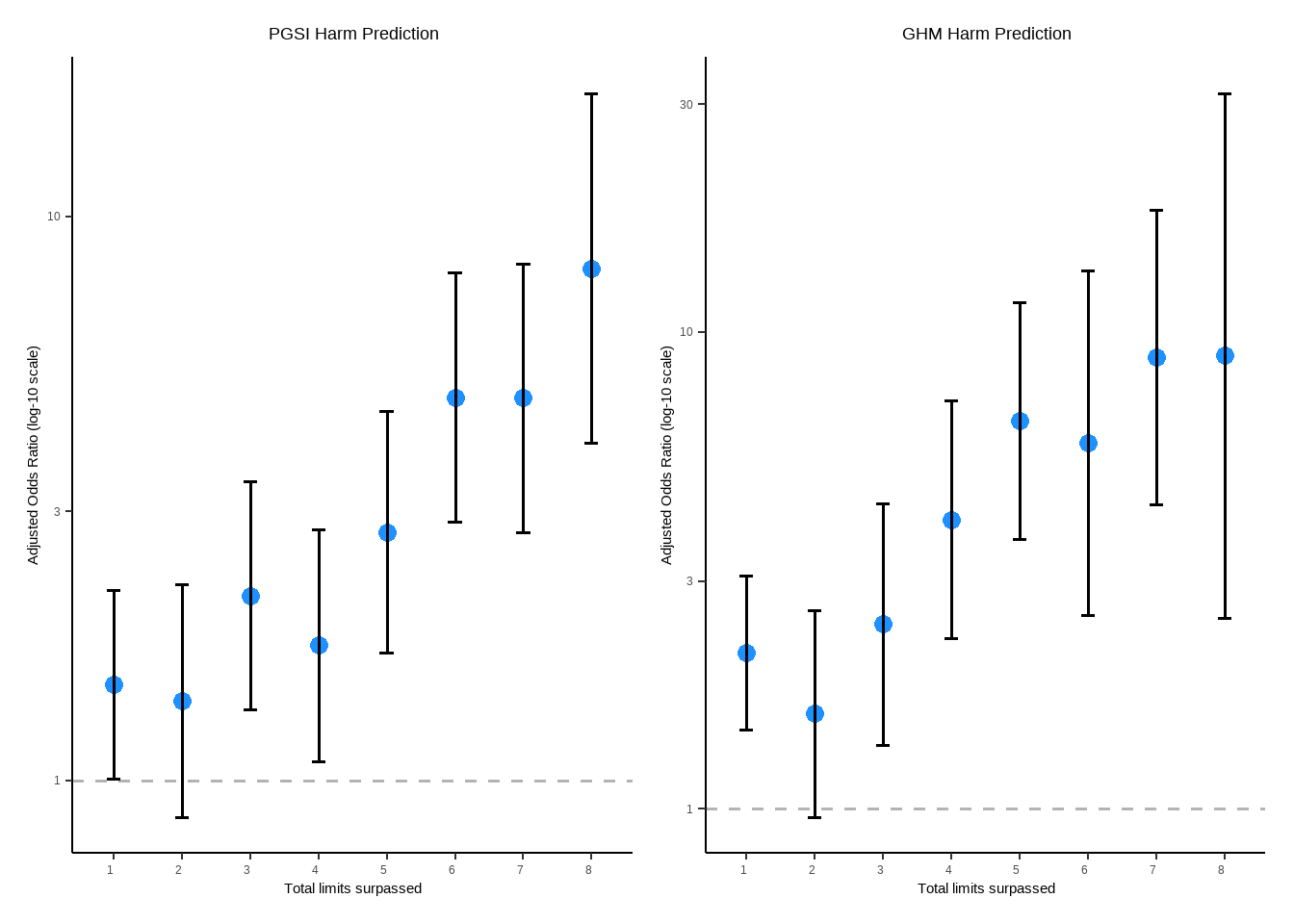
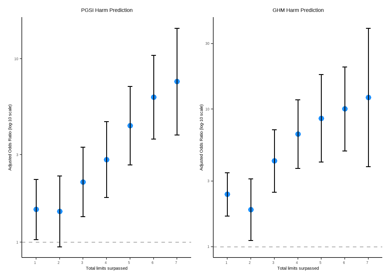
Finally, the test H3, we need to look at how the accumulation of limits past relates to harm. From our preregistration:
H3: Participants who surpass successively more of the eight newly derived low-risk in the six months preceding survey participation will have an increasingly greater odds of reporting the experience of harm after accounting for the impact of demographic factors (i.e., age, gender, employment status, and education level) on harm. That is, using logistic regression models with harm status as the outcome and the number of limits passed as an ordered categorical predictor variable, there will be a monotonic relationship between the number of limits passed and odds of harm (i.e., a larger odds ratio with each additional limit passed). [Limit evaluation: cumulative impact of limit breaches on harm status]
tbl_merge(tbls =list(tbl_weighted_lr_limit_count_PGSI, tbl_weighted_lr_limit_count_GHM),tab_spanner =c("**PGSI Status**", "**GHM Status**")) %>%as_gt() %>%tab_options(data_row.padding =px(1.5)) %>%tab_header(title ="Cumulative number of limits passed as a predictor of harm status (demographic-adjusted models)" )
Cumulative number of limits passed as a predictor of harm status (demographic-adjusted models)
Characteristic
PGSI Status
GHM Status
OR
95% CI
p-value
OR
95% CI
p-value
AGE
0.97
0.96, 0.98
<0.001
0.97
0.96, 0.98
<0.001
GENDER
Female
—
—
—
—
Male
1.71
1.19, 2.44
0.003
2.06
1.23, 3.47
0.006
Unknown
2.42
0.82, 7.17
0.11
2.03
0.56, 7.37
0.3
EMPLOYMENT_RECODED
Employed
—
—
—
—
Unemployed
1.37
0.74, 2.54
0.3
2.50
1.32, 4.72
0.005
Unknown
1.28
0.95, 1.71
0.10
0.96
0.66, 1.39
0.8
EDUCATION_NUM
0.92
0.85, 0.99
0.035
0.99
0.90, 1.08
0.8
Engages_in_other_forms
FALSE
—
—
—
—
TRUE
2.06
1.49, 2.85
<0.001
1.92
1.30, 2.82
<0.001
TOTAL_LIMITS_REACHED_PGSI
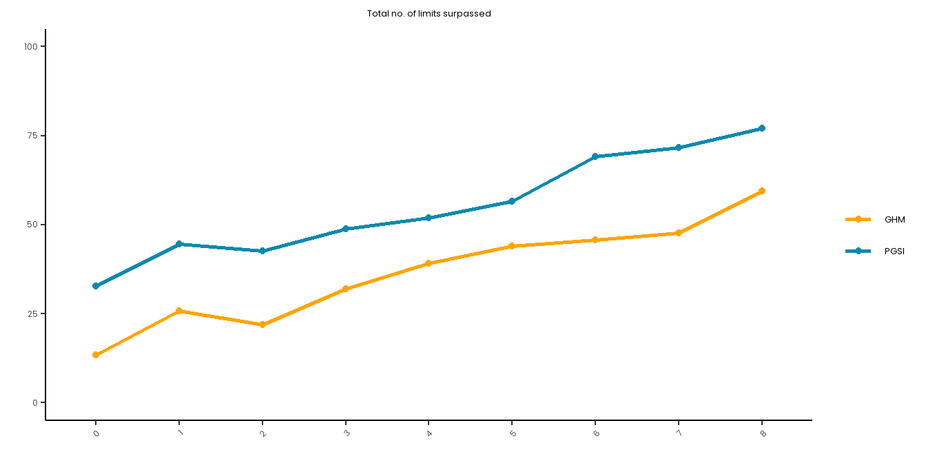
0
—
—
1
1.48
1.01, 2.18
0.046
2
1.39
0.86, 2.23
0.2
3
2.13
1.33, 3.39
0.002
4
1.74
1.08, 2.79
0.022
5
2.76
1.68, 4.52
<0.001
6
4.78
2.87, 7.97
<0.001
7
4.77
2.76, 8.24
<0.001
8
8.09
3.96, 16.5
<0.001
Null deviance
2,283
1,787
Null df
1,646
1,579
AIC
2,068
1,599
BIC
2,147
1,680
Deviance
2,029
1,562
Residual df
1,631
1,564
No. Obs.
1,647
1,580
TOTAL_LIMITS_REACHED_GHM
0
—
—
1
2.12
1.46, 3.08
<0.001
2
1.58
0.96, 2.60
0.071
3
2.44
1.36, 4.37
0.003
4
4.04
2.27, 7.16
<0.001
5
6.51
3.67, 11.6
<0.001
6
5.84
2.54, 13.4
<0.001
7
8.85
4.35, 18.0
<0.001
8
8.92
2.52, 31.7
<0.001
Abbreviations: CI = Confidence Interval, OR = Odds Ratio
Exponentiate coefficients and interpret them as odds-ratios in a data frame:
Show code
sumarisedORs_weighted_lr_limit_count_PGSI<-exp(cbind(OR =coef(weighted_lr_limit_count_PGSI), confint(weighted_lr_limit_count_PGSI)))sumarisedORs_weighted_lr_limit_count_PGSI %>%as.data.frame() %>%rownames_to_column() %>%mutate(across(c(OR, `2.5 %`, `97.5 %`), ~round(., 4))) %>%filter(str_detect(rowname, "TOTAL")) %>%mutate(rowname =str_remove(rowname, "TOTAL_LIMITS_REACHED_PGSI")) %>%gt() %>%tab_options(data_row.padding =px(1.5)) %>%tab_header(md("**Odds ratios with 95% CIs: Total number of limits passed (PGSI)**"), subtitle =NULL) %>%cols_label('2.5 %'="Lower CI: 2.5%",'97.5 %'="Upper CI: 97.5%")
Odds ratios with 95% CIs: Total number of limits passed (PGSI)
OR
Lower CI: 2.5%
Upper CI: 97.5%
1
1.4815
1.0077
2.1781
2
1.3868
0.8621
2.2309
3
2.1277
1.3338
3.3942
4
1.7375
1.0830
2.7876
5
2.7577
1.6837
4.5167
6
4.7812
2.8700
7.9652
7
4.7652
2.7551
8.2420
8
8.0913
3.9599
16.5330
Show code
sumarisedORs_weighted_lr_limit_count_GHM<-exp(cbind(OR =coef(weighted_lr_limit_count_GHM), confint(weighted_lr_limit_count_GHM)))sumarisedORs_weighted_lr_limit_count_GHM %>%as.data.frame() %>%rownames_to_column() %>%mutate(across(c(OR, `2.5 %`, `97.5 %`), ~round(., 4))) %>%filter(str_detect(rowname, "TOTAL")) %>%mutate(rowname =str_remove(rowname, "TOTAL_LIMITS_REACHED_GHM")) %>%gt() %>%tab_options(data_row.padding =px(1.5)) %>%tab_header(md("**Odds ratios with 95% CIs: Total number of limits passed (GHM)**"), subtitle =NULL) %>%cols_label('2.5 %'="Lower CI: 2.5%",'97.5 %'="Upper CI: 97.5%")
Odds ratios with 95% CIs: Total number of limits passed (GHM)
# NOTE: R2 is calculate as a proportion here and so in the paper we have multiplied it by 100 to form a percentage value
The model accounts for 19.0837288% of variance in PGSI harm rates.
Calculate Nagelkerke’s R squared for the GHM model:
Show code
NagelkerkeR2_weighted_lr_limit_count_PGSI<-NagelkerkeR2(weighted_lr_limit_count_GHM) %>%as.data.frame() %>%print() # NOTE: R2 is calculate as a proportion here and so in the paper we have multiplied it by 100 to form a percentage value
     N        R2
1 1580 0.1954103
The model accounts for 19.5410337% of variance in GHM harm rates.
tbl_merge(tbls =list(tbl_weighted_lr_limit_count_sans_freq_PGSI, tbl_weighted_lr_limit_count_sans_freq_GHM),tab_spanner =c("**PGSI Status**", "**GHM Status**")) %>%as_gt() %>%tab_options(data_row.padding =px(1.5)) %>%tab_header(title ="Cumulative number of limits passed as a predictor of harm status (demographic-adjusted models)" )
Cumulative number of limits passed as a predictor of harm status (demographic-adjusted models)
Characteristic
PGSI Status
GHM Status
OR
95% CI
p-value
OR
95% CI
p-value
AGE
0.97
0.96, 0.98
<0.001
0.97
0.96, 0.98
<0.001
GENDER
Female
—
—
—
—
Male
1.63
1.14, 2.33
0.008
1.99
1.18, 3.36
0.010
Unknown
2.22
0.77, 6.38
0.14
1.84
0.49, 6.92
0.4
EMPLOYMENT_RECODED
Employed
—
—
—
—
Unemployed
1.33
0.72, 2.47
0.4
2.59
1.38, 4.89
0.003
Unknown
1.28
0.95, 1.72
0.11
0.99
0.68, 1.44
>0.9
EDUCATION_NUM
0.92
0.85, 1.00
0.040
0.98
0.90, 1.08
0.7
Engages_in_other_forms
FALSE
—
—
—
—
TRUE
2.05
1.48, 2.85
<0.001
1.96
1.32, 2.91
<0.001
TOTAL_LIMITS_REACHED_PGSI_SANS_BET_FREQ
0
—
—
1
1.51
1.03, 2.20
0.033
2
1.47
0.94, 2.30
0.087
3
2.13
1.38, 3.30
<0.001
4
2.82
1.75, 4.55
<0.001
5
4.32
2.64, 7.07
<0.001
6
6.19
3.66, 10.5
<0.001
7
7.53
3.85, 14.7
<0.001
Null deviance
2,283
1,787
Null df
1,646
1,579
AIC
2,050
1,572
BIC
2,125
1,649
Deviance
2,014
1,538
Residual df
1,632
1,565
No. Obs.
1,647
1,580
TOTAL_LIMITS_REACHED_GHM_SANS_BET_FREQ
0
—
—
1
2.40
1.67, 3.46
<0.001
2
1.86
1.11, 3.11
0.018
3
4.21
2.49, 7.11
<0.001
4
6.60
3.72, 11.7
<0.001
5
8.59
4.14, 17.8
<0.001
6
10.0
4.98, 20.3
<0.001
7
12.2
3.83, 38.8
<0.001
Abbreviations: CI = Confidence Interval, OR = Odds Ratio
Exponentiate coefficients and interpret them as odds-ratios in a data frame:
Show code
sumarisedORs_weighted_lr_limit_count_sans_freq_PGSI<-exp(cbind(OR =coef(weighted_lr_limit_count_sans_freq_PGSI), confint(weighted_lr_limit_count_sans_freq_PGSI)))sumarisedORs_weighted_lr_limit_count_sans_freq_PGSI %>%as.data.frame() %>%rownames_to_column() %>%mutate(across(c(OR, `2.5 %`, `97.5 %`), ~round(., 4))) %>%filter(str_detect(rowname, "TOTAL")) %>%mutate(rowname =str_remove(rowname, "TOTAL_LIMITS_REACHED_PGSI_SANS_BET_FREQ")) %>%gt() %>%tab_options(data_row.padding =px(1.5)) %>%tab_header(md("**Odds ratios with 95% CIs: Total number of limits passed (PGSI)**"), subtitle =NULL) %>%cols_label('2.5 %'="Lower CI: 2.5%",'97.5 %'="Upper CI: 97.5%")
Odds ratios with 95% CIs: Total number of limits passed (PGSI)
OR
Lower CI: 2.5%
Upper CI: 97.5%
1
1.5091
1.0344
2.2019
2
1.4748
0.9447
2.3024
3
2.1318
1.3772
3.2998
4
2.8233
1.7532
4.5463
5
4.3227
2.6440
7.0671
6
6.1910
3.6586
10.4762
7
7.5273
3.8530
14.7055
Show code
sumarisedORs_weighted_lr_limit_count_sans_freq_GHM<-exp(cbind(OR =coef(weighted_lr_limit_count_sans_freq_GHM), confint(weighted_lr_limit_count_sans_freq_GHM)))sumarisedORs_weighted_lr_limit_count_sans_freq_GHM %>%as.data.frame() %>%rownames_to_column() %>%mutate(across(c(OR, `2.5 %`, `97.5 %`), ~round(., 4))) %>%filter(str_detect(rowname, "TOTAL")) %>%mutate(rowname =str_remove(rowname, "TOTAL_LIMITS_REACHED_GHM_SANS_BET_FREQ")) %>%gt() %>%tab_options(data_row.padding =px(1.5)) %>%tab_header(md("**Odds ratios with 95% CIs: Total number of limits passed (GHM)**"), subtitle =NULL) %>%cols_label('2.5 %'="Lower CI: 2.5%",'97.5 %'="Upper CI: 97.5%")
Odds ratios with 95% CIs: Total number of limits passed (GHM)
# NOTE: R2 is calculate as a proportion here and so in the paper we have multiplied it by 100 to form a percentage value
The model accounts for 20.0899743% of variance in PGSI harm rates.
Calculate Nagelkerke’s R squared for the GHM model:
Show code
NagelkerkeR2_weighted_lr_limit_count_sans_freq_PGSI<-NagelkerkeR2(weighted_lr_limit_count_sans_freq_GHM) %>%as.data.frame() %>%print() # NOTE: R2 is calculate as a proportion here and so in the paper we have multiplied it by 100 to form a percentage value
     N        R2
1 1580 0.2150508
The model accounts for 21.5050806% of variance in GHM harm rates.
ggsave("Figures/risk_curves_combined.pdf", plot = risk_curves_combined, height =240, width =170, units ="mm")
Phase 4: Demographic-adjusted predictive ability of old limits
First, to do this, we need to add new variables to the dataset indicating whether each participant exceeded the previous limits or not. The limits are taken from:
Dowling, N. A., Youssef, G. J., Greenwood, C., Merkouris, S. S., Suomi, A., & Room, R. (2021). The Identification of Low-risk Gambling Limits for Specific Gambling Activities. Journal of Gambling Studies, 38(2), Article 2. https://doi.org/10.1007/s10899-021-10036-z
These were the old limits:
Racing: No more than $288 spent per year [$24 per month]
Sports: No more than $400 spent per year [$33.3 per month]
Racing: No more than 0.55% of income spent on gambling
Sports: No more than 0.55% of income spent on gambling
Racing: No more than 15 active gambling days per year [1.25 per month]
Sports: No more than 14 active gambling days per year [1.17 per month]
Now add new variables for each of these which represent whether somebody passed or did not pass these limits:
For each of the old limit values, we need to compute the accuracy level if these were used to screen for harm status in our sample, as per H4.1 in our pre-reg:
“Our limits will be better at differentiating between harmed and unharmed participants in our sample compared to when limits for both horse/dog racing and sports/other events betting identified by Dowling et al. (2021) are used. Specifically, the accuracy (i.e., overall proportion of cases correctly classified) will be at least 5% greater when using our limits compared to the existing Dowling et al. limits [H4.1].”
We can compute many different types of performance metrics, including sensitivity (recall) and specificity as well as accuracy. First, we need to be able to compute all of the values that would go into a confusion matrix:
Now, perform logistic regressions to look at how well passing each limit predicts harm status after coding for demographic variables. We will need to run two models each time, one for the PGSI and one for the GHM.
For each model, we will run a function to produce plots showing diagnostic checks and then table regression outcomes together for the PGSI and GHM models, exponentiating betas into odds ratios.
tbl_merge(tbls =list(tbl_weighted_lr_freq_old_limit_PGSI_racing, tbl_weighted_lr_freq_old_limit_GHM_racing),tab_spanner =c("**PGSI Status**", "**GHM Status**")) %>%as_gt() %>%tab_options(data_row.padding =px(1.5)) %>%tab_header(title ="Dowling et al.'s (2021) gambling frequency limit for racing as a predictor of harm status" )
Dowling et al.'s (2021) gambling frequency limit for racing as a predictor of harm status
Characteristic
PGSI Status
GHM Status
OR
95% CI
p-value
OR
95% CI
p-value
AGE
0.97
0.96, 0.98
<0.001
0.97
0.96, 0.98
<0.001
GENDER
Female
—
—
—
—
Male
1.80
1.26, 2.56
0.001
2.35
1.40, 3.93
0.001
Unknown
2.39
0.92, 6.22
0.075
2.46
0.76, 7.99
0.13
EMPLOYMENT_RECODED
Employed
—
—
—
—
Unemployed
1.41
0.79, 2.51
0.2
2.87
1.56, 5.29
<0.001
Unknown
1.17
0.88, 1.56
0.3
0.99
0.70, 1.41
>0.9
EDUCATION_NUM
0.90
0.83, 0.97
0.007
0.97
0.89, 1.06
0.5
GAM_ACCOUNTS_NUM
1.35
1.23, 1.48
<0.001
1.33
1.19, 1.47
<0.001
Engages_in_other_forms
FALSE
—
—
—
—
TRUE
1.86
1.36, 2.54
<0.001
1.74
1.19, 2.52
0.004
OLD_LIMIT_RACING_FREQ
1.19
0.89, 1.58
0.2
1.29
0.92, 1.81
0.15
Null deviance
2,283
1,787
Null df
1,646
1,579
AIC
2,109
1,650
BIC
2,160
1,701
Deviance
2,086
1,627
Residual df
1,637
1,570
No. Obs.
1,647
1,580
Abbreviations: CI = Confidence Interval, OR = Odds Ratio
tbl_merge(tbls =list(tbl_weighted_lr_freq_old_limit_PGSI_sport, tbl_weighted_lr_freq_old_limit_GHM_sport),tab_spanner =c("**PGSI Status**", "**GHM Status**")) %>%as_gt() %>%tab_options(data_row.padding =px(1.5)) %>%tab_header(title ="Dowling et al.'s (2021) gambling frequency limit for sport as a predictor of harm status" )
Dowling et al.'s (2021) gambling frequency limit for sport as a predictor of harm status
Characteristic
PGSI Status
GHM Status
OR
95% CI
p-value
OR
95% CI
p-value
AGE
0.97
0.96, 0.98
<0.001
0.97
0.96, 0.98
<0.001
GENDER
Female
—
—
—
—
Male
1.80
1.26, 2.56
0.001
2.35
1.40, 3.93
0.001
Unknown
2.39
0.92, 6.22
0.074
2.46
0.76, 7.99
0.13
EMPLOYMENT_RECODED
Employed
—
—
—
—
Unemployed
1.41
0.79, 2.51
0.2
2.87
1.56, 5.28
<0.001
Unknown
1.17
0.88, 1.56
0.3
0.99
0.70, 1.42
>0.9
EDUCATION_NUM
0.90
0.83, 0.97
0.006
0.97
0.89, 1.06
0.5
GAM_ACCOUNTS_NUM
1.35
1.23, 1.48
<0.001
1.33
1.19, 1.47
<0.001
Engages_in_other_forms
FALSE
—
—
—
—
TRUE
1.86
1.36, 2.54
<0.001
1.74
1.19, 2.52
0.004
OLD_LIMIT_SPORT_FREQ
1.17
0.88, 1.56
0.3
1.28
0.91, 1.80
0.2
Null deviance
2,283
1,787
Null df
1,646
1,579
AIC
2,109
1,650
BIC
2,160
1,701
Deviance
2,086
1,627
Residual df
1,637
1,570
No. Obs.
1,647
1,580
Abbreviations: CI = Confidence Interval, OR = Odds Ratio
Interpretation in the context of H4.2: The odds ratio for PGSI harm was more than 0.1 larger for our limit for race and sports betting. For GHM harm, the odds ratios for our limits were larger, but only by 0.08 (Race betting) and 0.09 (Sports betting).
tbl_merge(tbls =list(tbl_weighted_lr_spend_old_limit_PGSI_racing, tbl_weighted_lr_spend_old_limit_GHM_racing),tab_spanner =c("**PGSI Status**", "**GHM Status**")) %>%as_gt() %>%tab_options(data_row.padding =px(1.5)) %>%tab_header(title ="Dowling et al.'s (2021) spend limit for racing as a predictor of harm status" )
Dowling et al.'s (2021) spend limit for racing as a predictor of harm status
Characteristic
PGSI Status
GHM Status
OR
95% CI
p-value
OR
95% CI
p-value
AGE
0.97
0.96, 0.98
<0.001
0.97
0.96, 0.98
<0.001
GENDER
Female
—
—
—
—
Male
1.74
1.22, 2.49
0.002
2.27
1.36, 3.79
0.002
Unknown
2.24
0.86, 5.85
0.10
2.32
0.72, 7.40
0.2
EMPLOYMENT_RECODED
Employed
—
—
—
—
Unemployed
1.46
0.81, 2.63
0.2
2.92
1.58, 5.39
<0.001
Unknown
1.16
0.87, 1.54
0.3
0.97
0.68, 1.39
0.9
EDUCATION_NUM
0.90
0.83, 0.97
0.007
0.97
0.89, 1.06
0.5
GAM_ACCOUNTS_NUM
1.34
1.22, 1.48
<0.001
1.32
1.19, 1.47
<0.001
Engages_in_other_forms
FALSE
—
—
—
—
TRUE
1.85
1.35, 2.53
<0.001
1.73
1.19, 2.51
0.004
OLD_LIMIT_RACING_SPEND
1.72
1.25, 2.37
<0.001
1.70
1.14, 2.52
0.009
Null deviance
2,283
1,787
Null df
1,646
1,579
AIC
2,096
1,643
BIC
2,147
1,694
Deviance
2,073
1,621
Residual df
1,637
1,570
No. Obs.
1,647
1,580
Abbreviations: CI = Confidence Interval, OR = Odds Ratio
tbl_merge(tbls =list(tbl_weighted_lr_spend_old_limit_PGSI_sport, tbl_weighted_lr_spend_old_limit_GHM_sport),tab_spanner =c("**PGSI Status**", "**GHM Status**")) %>%as_gt() %>%tab_options(data_row.padding =px(1.5)) %>%tab_header(title ="Dowling et al.'s (2021) spend limit for sport as a predictor of harm status" )
Dowling et al.'s (2021) spend limit for sport as a predictor of harm status
Characteristic
PGSI Status
GHM Status
OR
95% CI
p-value
OR
95% CI
p-value
AGE
0.97
0.96, 0.98
<0.001
0.97
0.96, 0.98
<0.001
GENDER
Female
—
—
—
—
Male
1.72
1.21, 2.45
0.003
2.22
1.33, 3.71
0.002
Unknown
2.19
0.83, 5.73
0.11
2.23
0.70, 7.15
0.2
EMPLOYMENT_RECODED
Employed
—
—
—
—
Unemployed
1.49
0.82, 2.68
0.2
2.97
1.59, 5.54
<0.001
Unknown
1.14
0.86, 1.52
0.4
0.95
0.67, 1.36
0.8
EDUCATION_NUM
0.90
0.83, 0.97
0.007
0.97
0.89, 1.06
0.5
GAM_ACCOUNTS_NUM
1.34
1.21, 1.47
<0.001
1.31
1.18, 1.46
<0.001
Engages_in_other_forms
FALSE
—
—
—
—
TRUE
1.87
1.36, 2.56
<0.001
1.75
1.20, 2.54
0.004
OLD_LIMIT_SPORT_SPEND
1.79
1.32, 2.43
<0.001
1.84
1.26, 2.69
0.002
Null deviance
2,283
1,787
Null df
1,646
1,579
AIC
2,092
1,639
BIC
2,143
1,690
Deviance
2,069
1,616
Residual df
1,637
1,570
No. Obs.
1,647
1,580
Abbreviations: CI = Confidence Interval, OR = Odds Ratio
Interpretation in the context of H4.2: The odds ratio for both PGSI harm and GHM harm was higher for our limits than these limits(both sport and race betting) by substantially more than 0.1 (10%).
Percentage of income spent
Racing & sports
The cut-off value is identical for sports and racing so there’s no need to do this twice:
tbl_merge(tbls =list(tbl_weighted_lr_income_percent_spend_old_limit_PGSI, tbl_weighted_lr_income_percent_spend_old_limit_GHM),tab_spanner =c("**PGSI Status**", "**GHM Status**")) %>%as_gt() %>%tab_options(data_row.padding =px(1.5)) %>%tab_header(title ="Dowling et al.'s (2021) percentage of income limit for racing and sport as a predictor of harm status" )
Dowling et al.'s (2021) percentage of income limit for racing and sport as a predictor of harm status
Characteristic
PGSI Status
GHM Status
OR
95% CI
p-value
OR
95% CI
p-value
AGE
0.97
0.96, 0.98
<0.001
0.98
0.96, 0.99
<0.001
GENDER
Female
—
—
—
—
Male
1.93
1.22, 3.04
0.005
2.76
1.46, 5.23
0.002
Unknown
3.99
1.10, 14.5
0.036
2.35
0.56, 9.79
0.2
EMPLOYMENT_RECODED
Employed
—
—
—
—
Unemployed
1.26
0.63, 2.51
0.5
2.14
1.05, 4.38
0.037
EDUCATION_NUM
0.91
0.83, 0.99
0.026
0.97
0.89, 1.07
0.6
GAM_ACCOUNTS_NUM
1.32
1.18, 1.49
<0.001
1.33
1.17, 1.51
<0.001
Engages_in_other_forms
FALSE
—
—
—
—
TRUE
1.89
1.30, 2.75
<0.001
1.76
1.15, 2.70
0.009
OLD_LIMIT_RACING_SPORT_INCOME_SPENT
2.04
1.47, 2.84
<0.001
2.19
1.47, 3.25
<0.001
Null deviance
1,527
1,288
Null df
1,054
1,054
AIC
1,391
1,189
BIC
1,433
1,232
Deviance
1,371
1,169
Residual df
1,046
1,046
No. Obs.
1,055
1,055
Abbreviations: CI = Confidence Interval, OR = Odds Ratio
Interpretation in the context of H4.2: The odds ratio for both PGSI harm and GHM harm was higher for our limits than these limits by substantially more than 0.1 (10%).
Phase 5: Rates of limit passing in different groups
Do some recoding of the data to get us the most simple categories for passing/not passing limits:
Show code
master_dataset_recoded_w_new_limits_post_survey <- master_dataset_recoded_w_new_limits %>%# Betting frequency:mutate(NEW_LIMIT_PGSI_BET_FREQ_POST_SURVEY =case_when( NEX_6M_MONTHLY_BET_FREQ_DAYS >round(optimal_limits %>%filter(Predictor =="PAS_6M_MONTHLY_BET_FREQ_DAYS") %>%pull(optimal_cutpoint_PGSI),0) ~1, NEX_6M_MONTHLY_BET_FREQ_DAYS <=round(optimal_limits %>%filter(Predictor =="PAS_6M_MONTHLY_BET_FREQ_DAYS") %>%pull(optimal_cutpoint_PGSI), 0) ~0,TRUE~NA_real_ )) %>%mutate(NEW_LIMIT_GHM_BET_FREQ_POST_SURVEY =case_when( NEX_6M_MONTHLY_BET_FREQ_DAYS >round(optimal_limits %>%filter(Predictor =="PAS_6M_MONTHLY_BET_FREQ_DAYS") %>%pull(optimal_cutpoint_GHM),0) ~1, NEX_6M_MONTHLY_BET_FREQ_DAYS <=round(optimal_limits %>%filter(Predictor =="PAS_6M_MONTHLY_BET_FREQ_DAYS") %>%pull(optimal_cutpoint_GHM), 0) ~0,TRUE~NA_real_ )) %>%# Check coding has worked:# select(NEX_6M_MONTHLY_BET_FREQ_DAYS,# NEW_LIMIT_PGSI_BET_FREQ_POST_SURVEY,# NEW_LIMIT_GHM_BET_FREQ_POST_SURVEY)# # Spend/turnover:mutate(NEW_LIMIT_PGSI_SPEND_POST_SURVEY =case_when( NEX_6M_MONTHLY_SPEND >250~1, NEX_6M_MONTHLY_SPEND <=250~0,TRUE~NA_real_ )) %>%mutate(NEW_LIMIT_GHM_SPEND_POST_SURVEY =case_when( NEX_6M_MONTHLY_SPEND >2100~1, NEX_6M_MONTHLY_SPEND <=2100~0,TRUE~NA_real_ )) %>%# Check coding has worked:# select(NEX_6M_MONTHLY_SPEND,# NEW_LIMIT_PGSI_SPEND_POST_SURVEY,# NEW_LIMIT_GHM_SPEND_POST_SURVEY)# Percentage of income spent:mutate(NEW_LIMIT_PGSI_INCOME_SPENT_POST_SURVEY =case_when( PERCENT_MON_INCOME_SPENT_MONTHLY_NEX_6M >round(optimal_limits %>%filter(Predictor =="PERCENT_MON_INCOME_SPENT_MONTHLY_PAS_6M") %>%pull(optimal_cutpoint_PGSI),0) ~1, PERCENT_MON_INCOME_SPENT_MONTHLY_NEX_6M <=round(optimal_limits %>%filter(Predictor =="PERCENT_MON_INCOME_SPENT_MONTHLY_PAS_6M") %>%pull(optimal_cutpoint_PGSI),0) ~0,TRUE~NA_real_ )) %>%mutate(NEW_LIMIT_GHM_INCOME_SPENT_POST_SURVEY =case_when( PERCENT_MON_INCOME_SPENT_MONTHLY_NEX_6M >round(optimal_limits %>%filter(Predictor =="PERCENT_MON_INCOME_SPENT_MONTHLY_PAS_6M") %>%pull(optimal_cutpoint_GHM),0) ~1, PERCENT_MON_INCOME_SPENT_MONTHLY_NEX_6M <=round(optimal_limits %>%filter(Predictor =="PERCENT_MON_INCOME_SPENT_MONTHLY_PAS_6M") %>%pull(optimal_cutpoint_GHM),0) ~0,TRUE~NA_real_ )) %>%# Check coding has worked:# select(PERCENT_MON_INCOME_SPENT_MONTHLY_NEX_6M,# NEW_LIMIT_GHM_INCOME_SPENT_POST_SURVEY,# NEW_LIMIT_PGSI_INCOME_SPENT_POST_SURVEY) %>%# print(n=100)# Number of sports/races bet on:mutate(NEW_LIMIT_PGSI_N_ACTIVITIES_POST_SURVEY =case_when( NEX_6M_N_ACTIVITIES >round(optimal_limits %>%filter(Predictor =="PAS_6M_N_ACTIVITIES") %>%pull(optimal_cutpoint_PGSI),0) ~1, NEX_6M_N_ACTIVITIES <=round(optimal_limits %>%filter(Predictor =="PAS_6M_N_ACTIVITIES") %>%pull(optimal_cutpoint_PGSI),0) ~0,TRUE~NA_real_ )) %>%mutate(NEW_LIMIT_GHM_N_ACTIVITIES_POST_SURVEY =case_when( NEX_6M_N_ACTIVITIES >round(optimal_limits %>%filter(Predictor =="PAS_6M_N_ACTIVITIES") %>%pull(optimal_cutpoint_GHM),0) ~1, NEX_6M_N_ACTIVITIES <=round(optimal_limits %>%filter(Predictor =="PAS_6M_N_ACTIVITIES") %>%pull(optimal_cutpoint_GHM),0) ~0,TRUE~NA_real_ )) %>%# Check coding has worked:# select(NEX_6M_N_ACTIVITIES,# NEW_LIMIT_PGSI_N_ACTIVITIES_POST_SURVEY,# NEW_LIMIT_GHM_N_ACTIVITIES_POST_SURVEY) %>%# print(n=100)# Deposit frequency:mutate(NEW_LIMIT_PGSI_DEPOSIT_FREQ_POST_SURVEY =case_when( NEX_6M_MONTHLY_DEPOSIT_FREQ >round(optimal_limits %>%filter(Predictor =="PAS_6M_MONTHLY_DEPOSIT_FREQ") %>%pull(optimal_cutpoint_PGSI),0) ~1, NEX_6M_MONTHLY_DEPOSIT_FREQ <=round(optimal_limits %>%filter(Predictor =="PAS_6M_MONTHLY_DEPOSIT_FREQ") %>%pull(optimal_cutpoint_PGSI),0) ~0,TRUE~NA_real_ )) %>%mutate(NEW_LIMIT_GHM_DEPOSIT_FREQ_POST_SURVEY =case_when( NEX_6M_MONTHLY_DEPOSIT_FREQ >round(optimal_limits %>%filter(Predictor =="PAS_6M_MONTHLY_DEPOSIT_FREQ") %>%pull(optimal_cutpoint_GHM),0) ~1, NEX_6M_MONTHLY_DEPOSIT_FREQ <=round(optimal_limits %>%filter(Predictor =="PAS_6M_MONTHLY_DEPOSIT_FREQ") %>%pull(optimal_cutpoint_GHM),0) ~0,TRUE~NA_real_ )) %>%# Check coding has worked:# select(NEX_6M_MONTHLY_DEPOSIT_FREQ,# NEW_LIMIT_PGSI_DEPOSIT_FREQ_POST_SURVEY,# NEW_LIMIT_GHM_DEPOSIT_FREQ_POST_SURVEY) %>%# print(n=100)# Deposit amount:mutate(NEW_LIMIT_PGSI_DEPOSIT_AMOUNT_POST_SURVEY =case_when( NEX_6M_MONTHLY_DEPOSIT_AMOUNT >round(optimal_limits %>%filter(Predictor =="PAS_6M_MONTHLY_DEPOSIT_AMOUNT") %>%pull(optimal_cutpoint_PGSI),0) ~1, NEX_6M_MONTHLY_DEPOSIT_AMOUNT <=round(optimal_limits %>%filter(Predictor =="PAS_6M_MONTHLY_DEPOSIT_AMOUNT") %>%pull(optimal_cutpoint_PGSI),0) ~0,TRUE~NA_real_ )) %>%mutate(NEW_LIMIT_GHM_DEPOSIT_AMOUNT_POST_SURVEY =case_when( NEX_6M_MONTHLY_DEPOSIT_AMOUNT >=900~1, NEX_6M_MONTHLY_DEPOSIT_AMOUNT <900~0,TRUE~NA_real_ )) %>%# Check coding has worked:# select(NEX_6M_MONTHLY_DEPOSIT_AMOUNT,# NEW_LIMIT_PGSI_DEPOSIT_AMOUNT_POST_SURVEY,# NEW_LIMIT_GHM_DEPOSIT_AMOUNT_POST_SURVEY) %>%# print(n=100)# Percentage of income deposited:mutate(NEW_LIMIT_PGSI_INCOME_DEPOSITED_POST_SURVEY =case_when( PERCENT_MON_INCOME_DEPOSIT_MONTHLY_NEX_6M >round(optimal_limits %>%filter(Predictor =="PERCENT_MON_INCOME_DEPOSIT_MONTHLY_PAS_6M") %>%pull(optimal_cutpoint_PGSI),0) ~1, PERCENT_MON_INCOME_DEPOSIT_MONTHLY_NEX_6M <=round(optimal_limits %>%filter(Predictor =="PERCENT_MON_INCOME_DEPOSIT_MONTHLY_PAS_6M") %>%pull(optimal_cutpoint_PGSI),0) ~0,TRUE~NA_real_ )) %>%mutate(NEW_LIMIT_GHM_INCOME_DEPOSITED_POST_SURVEY =case_when( PERCENT_MON_INCOME_DEPOSIT_MONTHLY_NEX_6M >round(optimal_limits %>%filter(Predictor =="PERCENT_MON_INCOME_DEPOSIT_MONTHLY_PAS_6M") %>%pull(optimal_cutpoint_GHM),0) ~1, PERCENT_MON_INCOME_DEPOSIT_MONTHLY_NEX_6M <=round(optimal_limits %>%filter(Predictor =="PERCENT_MON_INCOME_DEPOSIT_MONTHLY_PAS_6M") %>%pull(optimal_cutpoint_GHM),0) ~0,TRUE~NA_real_ )) %>%# Check coding has worked:# select(PERCENT_MON_INCOME_DEPOSIT_MONTHLY_NEX_6M,# NEW_LIMIT_PGSI_INCOME_DEPOSITED_POST_SURVEY,# NEW_LIMIT_GHM_INCOME_DEPOSITED_POST_SURVEY)%>%# print(n=100)# Number of gambling accounts:mutate(NEW_LIMIT_PGSI_GAM_ACCOUNTS_POST_SURVEY =case_when( # this is obviously the same as pre-survey, but re-doing it here just helps with totals computed below) GAM_ACCOUNTS_NUM >3~1, GAM_ACCOUNTS_NUM <=3~0,TRUE~NA_real_ )) %>%# Number of gambling accounts proposed:mutate(NEW_LIMIT_PGSI_GAM_ACCOUNTS_PROPOSED =case_when( # this is obviously the same as pre-survey, but re-doing it here just helps with totals computed below) GAM_ACCOUNTS_NUM >2~1, GAM_ACCOUNTS_NUM <=2~0,TRUE~NA_real_ )) %>%# recode outcome variables for simplicity of interpretation in regression models:mutate(PGSI_STATUS =case_when(PGSI_STATUS ==1~"Harm", PGSI_STATUS ==0~"No harm",TRUE~NA)) %>%mutate(GHM_STATUS =case_when(GHM_STATUS ==1~"Harm", GHM_STATUS ==0~"No harm",TRUE~NA)) %>%# Calculate the total no. of limits reached:mutate(TOTAL_LIMITS_REACHED_POST_SURVEY_PGSI =rowSums(select(., matches("PGSI.*_POST_SURVEY$")), na.rm =TRUE)) %>%# Make it so that the variable recognises zero values, even though there are none yet.# mutate(# TOTAL_LIMITS_REACHED_POST_SURVEY_PGSI = factor(TOTAL_LIMITS_REACHED_POST_SURVEY_PGSI),# TOTAL_LIMITS_REACHED_POST_SURVEY_PGSI = fct_expand(TOTAL_LIMITS_REACHED_POST_SURVEY_PGSI, "0"),# TOTAL_LIMITS_REACHED_POST_SURVEY_PGSI = relevel(TOTAL_LIMITS_REACHED_POST_SURVEY_PGSI, ref = "0")# ) %>%# # now set the reference level to 0:# mutate(TOTAL_LIMITS_REACHED_POST_SURVEY_PGSI = relevel(as.factor(TOTAL_LIMITS_REACHED_POST_SURVEY_PGSI), ref = "0")) %>%select(CLIENT_ID, ELIGIBLE_SURVEY_SAMPLE_WEIGHTS, PERCENT_MON_INCOME_DEPOSIT_MONTHLY_PAS_6M, GHM_STATUS, PGSI_STATUS, NEW_LIMIT_PGSI_BET_FREQ, NEW_LIMIT_GHM_BET_FREQ, NEW_LIMIT_PGSI_BET_FREQ_POST_SURVEY, NEW_LIMIT_GHM_BET_FREQ_POST_SURVEY, NEW_LIMIT_PGSI_SPEND, NEW_LIMIT_GHM_SPEND, NEW_LIMIT_PGSI_SPEND_POST_SURVEY, NEW_LIMIT_GHM_SPEND_POST_SURVEY, NEW_LIMIT_PGSI_INCOME_SPENT, NEW_LIMIT_GHM_INCOME_SPENT, NEW_LIMIT_PGSI_INCOME_SPENT_POST_SURVEY, NEW_LIMIT_GHM_INCOME_SPENT_POST_SURVEY, NEW_LIMIT_PGSI_N_ACTIVITIES, NEW_LIMIT_GHM_N_ACTIVITIES, NEW_LIMIT_PGSI_N_ACTIVITIES_POST_SURVEY, NEW_LIMIT_GHM_N_ACTIVITIES_POST_SURVEY, NEW_LIMIT_PGSI_DEPOSIT_FREQ, NEW_LIMIT_GHM_DEPOSIT_FREQ, NEW_LIMIT_PGSI_DEPOSIT_FREQ_POST_SURVEY, NEW_LIMIT_GHM_DEPOSIT_FREQ_POST_SURVEY, NEW_LIMIT_PGSI_DEPOSIT_AMOUNT, NEW_LIMIT_GHM_DEPOSIT_AMOUNT, NEW_LIMIT_PGSI_DEPOSIT_AMOUNT_POST_SURVEY, NEW_LIMIT_GHM_DEPOSIT_AMOUNT_POST_SURVEY, NEW_LIMIT_PGSI_INCOME_DEPOSITED, NEW_LIMIT_GHM_INCOME_DEPOSITED, NEW_LIMIT_PGSI_INCOME_DEPOSITED_POST_SURVEY, NEW_LIMIT_GHM_INCOME_DEPOSITED_POST_SURVEY, NEW_LIMIT_PGSI_GAM_ACCOUNTS_POST_SURVEY, NEW_LIMIT_PGSI_GAM_ACCOUNTS_PROPOSED, TOTAL_LIMITS_REACHED_POST_SURVEY_PGSI ) %>%filter(!is.na(TOTAL_LIMITS_REACHED_POST_SURVEY_PGSI)) %>%filter(!is.na(PERCENT_MON_INCOME_DEPOSIT_MONTHLY_PAS_6M))
Note that this sample purposely excludes anyone who has any missing data in any of our relevant variables to ensure a consistent sample is used to compute rates across the different behavioural indicators. ### Re-weighting
We need to update the the survey design object with new variables:
tbl_merge(tbls =list(pre_survey_passing_rates, post_survey_passing_rates),tab_spanner =c("**Six months pre-survey**","**Six months post-survey**")) %>%as_gt() %>%tab_row_group(label ="Number of active gambling accounts (12 months pre-survey)", rows =15:16 ) %>%tab_row_group(label ="% monthly income deposited per month", rows =13:14 ) %>%tab_row_group(label ="Monthly deposit amount", rows =11:12 ) %>%tab_row_group(label ="Monthly deposit frequency", rows =9:10 ) %>%tab_row_group(label ="Number of different activities bet on", rows =7:8 ) %>%tab_row_group(label ="% monthly income spent per month", rows =5:6 ) %>%tab_row_group(label ="Spend per month", rows =3:4 ) %>%tab_row_group(label ="Betting days per month", rows =1:2 ) %>%tab_options(data_row.padding =px(2),row_group.padding =px(2)) %>%tab_header("Table 5. Number and percentage of customers above each new optimal limit in the six months before and after participation: Overall rates and grouped by PGSI and GHM status") %>%tab_footnote( "" )
Table 5. Number and percentage of customers above each new optimal limit in the six months before and after participation: Overall rates and grouped by PGSI and GHM status
Characteristic
Six months pre-survey
Six months post-survey
Overall1
Harm1
No harm1
Harm1
No harm1
Overall1
Harm1
No harm1
Harm1
No harm1
Betting days per month
NEW_LIMIT_PGSI_BET_FREQ
521 (49%)
316 (54%)
205 (43%)
190 (56%)
331 (46%)
475 (45%)
275 (47%)
200 (42%)
171 (51%)
304 (42%)
NEW_LIMIT_GHM_BET_FREQ
383 (36%)
237 (41%)
146 (31%)
141 (42%)
242 (34%)
342 (32%)
209 (36%)
133 (28%)
124 (37%)
218 (30%)
Spend per month
NEW_LIMIT_PGSI_SPEND
609 (58%)
396 (68%)
213 (45%)
252 (75%)
357 (50%)
549 (52%)
352 (61%)
197 (42%)
224 (66%)
325 (45%)
NEW_LIMIT_GHM_SPEND
314 (30%)
223 (38%)
91 (19%)
153 (45%)
161 (22%)
256 (24%)
179 (31%)
77 (16%)
116 (34%)
140 (19%)
% monthly income spent per month
NEW_LIMIT_PGSI_INCOME_SPENT
494 (47%)
341 (59%)
153 (32%)
228 (68%)
266 (37%)
439 (42%)
293 (50%)
146 (31%)
193 (57%)
246 (34%)
NEW_LIMIT_GHM_INCOME_SPENT
434 (41%)
307 (53%)
127 (27%)
213 (63%)
221 (31%)
383 (36%)
262 (45%)
121 (26%)
174 (52%)
209 (29%)
Number of different activities bet on
NEW_LIMIT_PGSI_N_ACTIVITIES
470 (45%)
306 (53%)
164 (35%)
191 (57%)
279 (39%)
422 (40%)
279 (48%)
143 (30%)
175 (52%)
247 (34%)
NEW_LIMIT_GHM_N_ACTIVITIES
366 (35%)
246 (42%)
120 (25%)
150 (45%)
216 (30%)
317 (30%)
215 (37%)
102 (22%)
138 (41%)
179 (25%)
Monthly deposit frequency
NEW_LIMIT_PGSI_DEPOSIT_FREQ
473 (45%)
340 (59%)
133 (28%)
224 (66%)
249 (35%)
390 (37%)
276 (48%)
114 (24%)
181 (54%)
209 (29%)
NEW_LIMIT_GHM_DEPOSIT_FREQ
297 (28%)
226 (39%)
71 (15%)
153 (45%)
144 (20%)
222 (21%)
166 (29%)
56 (12%)
107 (32%)
115 (16%)
Monthly deposit amount
NEW_LIMIT_PGSI_DEPOSIT_AMOUNT
623 (59%)
419 (72%)
204 (43%)
266 (79%)
357 (50%)
514 (49%)
344 (59%)
170 (36%)
215 (64%)
299 (42%)
NEW_LIMIT_GHM_DEPOSIT_AMOUNT
312 (30%)
226 (39%)
86 (18%)
155 (46%)
157 (22%)
209 (20%)
149 (26%)
60 (13%)
94 (28%)
115 (16%)
% monthly income deposited per month
NEW_LIMIT_PGSI_INCOME_DEPOSITED
495 (47%)
354 (61%)
141 (30%)
233 (69%)
262 (36%)
393 (37%)
275 (47%)
118 (25%)
182 (54%)
211 (29%)
NEW_LIMIT_GHM_INCOME_DEPOSITED
313 (30%)
231 (40%)
82 (17%)
167 (50%)
146 (20%)
213 (20%)
157 (27%)
56 (12%)
102 (30%)
111 (15%)
Number of active gambling accounts (12 months pre-survey)
NEW_LIMIT_PGSI_GAM_ACCOUNTS_POST_SURVEY
321 (30%)
208 (36%)
113 (24%)
134 (40%)
187 (26%)
321 (30%)
208 (36%)
113 (24%)
134 (40%)
187 (26%)
NEW_LIMIT_PGSI_GAM_ACCOUNTS_PROPOSED
589 (56%)
369 (64%)
220 (46%)
229 (68%)
360 (50%)
589 (56%)
369 (64%)
220 (46%)
229 (68%)
360 (50%)
1 n (unweighted) (% (unweighted))
Weighted percentages added
Remake tables but with unweighted and weighted percentages included:
tbl_merge(tbls =list(pre_survey_passing_rates, post_survey_passing_rates),tab_spanner =c("**Six months pre-survey**","**Six months post-survey**")) %>%as_gt() %>%tab_row_group(label ="Number of active gambling accounts (12 months pre-survey)", rows =15 ) %>%tab_row_group(label ="% monthly income deposited per month", rows =13:14 ) %>%tab_row_group(label ="Monthly deposit amount", rows =11:12 ) %>%tab_row_group(label ="Monthly deposit frequency", rows =9:10 ) %>%tab_row_group(label ="Number of different activities bet on", rows =7:8 ) %>%tab_row_group(label ="% monthly income spent per month", rows =5:6 ) %>%tab_row_group(label ="Spend per month", rows =3:4 ) %>%tab_row_group(label ="Betting days per month", rows =1:2 ) %>%tab_options(data_row.padding =px(2),row_group.padding =px(2)) %>%tab_header("Supplemental Table 2. Number and percentage (unweighted; weighted) of customers above each new optimal limit in the six months before and after participation: Overall rates and grouped by PGSI and GHM status") %>%tab_footnote( "" )
Supplemental Table 2. Number and percentage (unweighted; weighted) of customers above each new optimal limit in the six months before and after participation: Overall rates and grouped by PGSI and GHM status
Characteristic
Six months pre-survey
Six months post-survey
Overall1
Harm1
No harm1
Harm1
No harm1
Overall2
Harm2
No harm2
Harm2
No harm2
Betting days per month
NEW_LIMIT_PGSI_BET_FREQ
475 (45%; 37%)
275 (47%; 38%)
200 (42%; 36%)
171 (51%; 43%)
304 (42%; 35%)
475 (37%)
275 (38%)
200 (36%)
171 (43%)
304 (35%)
NEW_LIMIT_GHM_BET_FREQ
342 (32%; 24%)
209 (36%; 27%)
133 (28%; 22%)
124 (37%; 29%)
218 (30%; 23%)
342 (24%)
209 (27%)
133 (22%)
124 (29%)
218 (23%)
Spend per month
NEW_LIMIT_PGSI_SPEND
549 (52%; 40%)
352 (61%; 48%)
197 (42%; 33%)
224 (66%; 55%)
325 (45%; 35%)
549 (40%)
352 (48%)
197 (33%)
224 (55%)
325 (35%)
NEW_LIMIT_GHM_SPEND
256 (24%; 9.7%)
179 (31%; 14%)
77 (16%; 5.7%)
116 (34%; 18%)
140 (19%; 6.5%)
256 (9.7%)
179 (14%)
77 (5.7%)
116 (18%)
140 (6.5%)
% monthly income spent per month
NEW_LIMIT_PGSI_INCOME_SPENT
439 (42%; 29%)
293 (50%; 36%)
146 (31%; 21%)
193 (57%; 44%)
246 (34%; 23%)
439 (29%)
293 (36%)
146 (21%)
193 (44%)
246 (23%)
NEW_LIMIT_GHM_INCOME_SPENT
383 (36%; 22%)
262 (45%; 30%)
121 (26%; 15%)
174 (52%; 38%)
209 (29%; 17%)
383 (22%)
262 (30%)
121 (15%)
174 (38%)
209 (17%)
Number of different activities bet on
NEW_LIMIT_PGSI_N_ACTIVITIES
422 (40%; 33%)
279 (48%; 42%)
143 (30%; 25%)
175 (52%; 47%)
247 (34%; 28%)
422 (33%)
279 (42%)
143 (25%)
175 (47%)
247 (28%)
NEW_LIMIT_GHM_N_ACTIVITIES
317 (30%; 24%)
215 (37%; 31%)
102 (22%; 17%)
138 (41%; 35%)
179 (25%; 19%)
317 (24%)
215 (31%)
102 (17%)
138 (35%)
179 (19%)
Monthly deposit frequency
NEW_LIMIT_PGSI_DEPOSIT_FREQ
390 (37%; 27%)
276 (48%; 38%)
114 (24%; 15%)
181 (54%; 47%)
209 (29%; 19%)
390 (27%)
276 (38%)
114 (15%)
181 (47%)
209 (19%)
NEW_LIMIT_GHM_DEPOSIT_FREQ
222 (21%; 11%)
166 (29%; 18%)
56 (12%; 4.1%)
107 (32%; 23%)
115 (16%; 6.6%)
222 (11%)
166 (18%)
56 (4.1%)
107 (23%)
115 (6.6%)
Monthly deposit amount
NEW_LIMIT_PGSI_DEPOSIT_AMOUNT
514 (49%; 39%)
344 (59%; 50%)
170 (36%; 28%)
215 (64%; 56%)
299 (42%; 32%)
514 (39%)
344 (50%)
170 (28%)
215 (56%)
299 (32%)
NEW_LIMIT_GHM_DEPOSIT_AMOUNT
209 (20%; 6.5%)
149 (26%; 10%)
60 (13%; 2.8%)
94 (28%; 13%)
115 (16%; 4.1%)
209 (6.5%)
149 (10%)
60 (2.8%)
94 (13%)
115 (4.1%)
% monthly income deposited per month
NEW_LIMIT_PGSI_INCOME_DEPOSITED
393 (37%; 25%)
275 (47%; 36%)
118 (25%; 15%)
182 (54%; 45%)
211 (29%; 18%)
393 (25%)
275 (36%)
118 (15%)
182 (45%)
211 (18%)
NEW_LIMIT_GHM_INCOME_DEPOSITED
213 (20%; 7.4%)
157 (27%; 12%)
56 (12%; 2.5%)
102 (30%; 17%)
111 (15%; 3.8%)
213 (7.4%)
157 (12%)
56 (2.5%)
102 (17%)
111 (3.8%)
Number of active gambling accounts (12 months pre-survey)
NEW_LIMIT_PGSI_GAM_ACCOUNTS_POST_SURVEY
321 (30%; 30%)
208 (36%; 37%)
113 (24%; 22%)
134 (40%; 40%)
187 (26%; 26%)
321 (30%)
208 (37%)
113 (22%)
134 (40%)
187 (26%)
NEW_LIMIT_PGSI_GAM_ACCOUNTS_PROPOSED
589 (56%; 55%)
369 (64%; 65%)
220 (46%; 45%)
229 (68%; 70%)
360 (50%; 50%)
589 (55%)
369 (65%)
220 (45%)
229 (70%)
360 (50%)
1 n (unweighted) (% (unweighted); %)
2 n (unweighted) (%)
EXPLORATORY ANALYSES
Subset of predictors
Which model most effectively and efficiently predicts PGSI status (i.e., which combination of the variables are most useful; noting that this doesn’t consider demographic or other gambling controls):
Show code
master_dataset_recoded_w_new_limits_filtered_NAs <- master_dataset_recoded_w_new_limits %>%filter(!is.na(NEW_LIMIT_PGSI_INCOME_SPENT)) %>%as.data.frame()data_subset <- master_dataset_recoded_w_new_limits_filtered_NAs[, c("PGSI_STATUS", "NEW_LIMIT_PGSI_SPEND", "NEW_LIMIT_PGSI_INCOME_SPENT", "NEW_LIMIT_PGSI_N_ACTIVITIES", "NEW_LIMIT_PGSI_DEPOSIT_FREQ", "NEW_LIMIT_PGSI_DEPOSIT_AMOUNT", "NEW_LIMIT_PGSI_INCOME_DEPOSITED", "NEW_LIMIT_PGSI_GAM_ACCOUNTS")]best_model <-bestglm(data_subset, IC ="AIC",family = binomial)# The output provides the best model based on AICprint(best_model$BestModel)
Call:  glm(formula = y ~ ., family = family, data = Xi, weights = weights)

Coefficients:
                  (Intercept)                    PGSI_STATUS
                      -0.2720                         0.6763
  NEW_LIMIT_PGSI_DEPOSIT_FREQ  NEW_LIMIT_PGSI_DEPOSIT_AMOUNT
                      -0.4973                         0.6205

Degrees of Freedom: 1054 Total (i.e. Null);  1051 Residual
Null Deviance:      1448
Residual Deviance: 1405     AIC: 1413
SPECIFIC LIMITS FOR YOUNG PEOPLE
Phase 2 young people: Identifying optimal limits for behavioural indicators
master_dataset_recoded_under26s %>%tbl_summary(include =c(PGSI_STATUS,GHM_STATUS),missing ="no") %>%modify_header(all_stat_cols() ~"**{level}**") %>%as_gt() %>%tab_options(data_row.padding =px(1.5)) %>%tab_header(title ="Rates of harm for GHM & PGSI",subtitle ="25s and under only (unweighted)" )
Rates of harm for GHM & PGSI
25s and under only (unweighted)
Characteristic
Overall1
PGSI_STATUS
Harm
159 (67%)
No harm
80 (33%)
GHM_STATUS
Harm
87 (41%)
No harm
125 (59%)
1 n (%)
Show code
master_dataset_recoded_under26s %>%tbl_summary(include =c(GHM_STATUS),by = PGSI_STATUS,missing ="no") %>%modify_header(all_stat_cols() ~"**{level}**") %>%# show_header_names() modify_header(stat_1 ="PGSI: Harm",stat_2 ="PGSI: No harm") %>%as_gt() %>%tab_options(data_row.padding =px(1.5)) %>%tab_header(title ="Rates of harm for GHM grouped by PGSI status",subtitle ="25s and under only (unweighted)" )
Rates of harm for GHM grouped by PGSI status
25s and under only (unweighted)
Characteristic
PGSI: Harm1
PGSI: No harm1
GHM_STATUS
Harm
83 (57%)
4 (6.0%)
No harm
62 (43%)
63 (94%)
1 n (%)
Select limits
Because of the extensive bootstrapping required for the three approaches for eight different behavioural indicators, the code below takes quite some time to run and has been commented out to save time each time the script runs and document knits. The outcomes from the bootstrapping were saved to a data file which is loaded in at the end of this process.
# # # First join and then save all outcomes as a dataset for easy retrieval later on:# AUC_limit_outcome_data <- bind_rows(# PAS_6M_MONTHLY_BET_FREQ_DAYS_AUC_Youden,# PAS_6M_MONTHLY_BET_FREQ_DAYS_AUC_Sensitivity,# PAS_6M_MONTHLY_BET_FREQ_DAYS_AUC_Specificity,# PAS_6M_MONTHLY_SPEND_AUC_Youden,# PAS_6M_MONTHLY_SPEND_AUC_Sensitivity,# PAS_6M_MONTHLY_SPEND_AUC_Specificity,# PERCENT_MON_INCOME_SPENT_MONTHLY_PAS_6M_AUC_Youden,# PERCENT_MON_INCOME_SPENT_MONTHLY_PAS_6M_AUC_Sensitivity,# PERCENT_MON_INCOME_SPENT_MONTHLY_PAS_6M_AUC_Specificity,# PAS_6M_N_ACTIVITIES_AUC_Youden,# PAS_6M_N_ACTIVITIES_AUC_Sensitivity,# PAS_6M_N_ACTIVITIES_AUC_Specificity,# PAS_6M_MONTHLY_DEPOSIT_FREQ_AUC_Youden,# PAS_6M_MONTHLY_DEPOSIT_FREQ_AUC_Sensitivity,# PAS_6M_MONTHLY_DEPOSIT_FREQ_AUC_Specificity,# PAS_6M_MONTHLY_DEPOSIT_AMOUNT_AUC_Youden,# PAS_6M_MONTHLY_DEPOSIT_AMOUNT_AUC_Sensitivity,# PAS_6M_MONTHLY_DEPOSIT_AMOUNT_AUC_Specificity,# PERCENT_MON_INCOME_DEPOSIT_MONTHLY_PAS_6M_AUC_Youden,# PERCENT_MON_INCOME_DEPOSIT_MONTHLY_PAS_6M_AUC_Sensitivity,# PERCENT_MON_INCOME_DEPOSIT_MONTHLY_PAS_6M_AUC_Specificity,# GAM_ACCOUNTS_AUC_Youden,# GAM_ACCOUNTS_AUC_Sensitivity,# GAM_ACCOUNTS_AUC_Specificity# ) %>%# mutate_if(is.numeric, round, 3)# # write.csv(AUC_limit_outcome_data,# "R Data files/AUC_limit_outcome_data_young_people.csv",# row.names=FALSE)# Read in outcome data:AUC_limit_outcome_data_young_people<-read.csv("R Data files/AUC_limit_outcome_data_young_people.csv")# Table them:AUC_limit_outcome_data_young_people %>%gt() %>%tab_options(data_row.padding =px(1.5))%>%tab_header(title ="Supplemental Table 3. Performance metrics for all cut-off points for all behavioural indicators: Specific to those aged under 26" )
Supplemental Table 3. Performance metrics for all cut-off points for all behavioural indicators: Specific to those aged under 26
predictor
optimal_cutpoint_PGSI
AUC_PGSI
sensitivity_PGSI
specificity_PGSI
acc_PGSI
Metric_maximised
X95.CIs_PGSI
optimal_cutpoint_GHM
AUC_GHM
sensitivity_GHM
specificity_GHM
acc_GHM
X95.CIs_GHM
method
PAS_6M_MONTHLY_BET_FREQ_DAYS
2.653
0.575
0.686
0.475
0.615
Youden
0.497, 0.651
3.461
0.589
0.713
0.488
0.580
0.514, 0.664
NA
PAS_6M_MONTHLY_BET_FREQ_DAYS
3.624
0.575
0.623
0.525
0.590
Sensitivity
0.496, 0.654
3.817
0.589
0.678
0.512
0.580
0.512, 0.668
NA
PAS_6M_MONTHLY_BET_FREQ_DAYS
5.101
0.575
0.509
0.613
0.544
Specificity
0.493, 0.654
6.081
0.589
0.494
0.648
0.585
0.516, 0.666
maximize_boot_metric
PAS_6M_MONTHLY_SPEND
116.285
0.597
0.692
0.500
0.628
Youden
0.516, 0.677
354.345
0.599
0.598
0.616
0.608
0.518, 0.673
NA
PAS_6M_MONTHLY_SPEND
135.708
0.597
0.679
0.512
0.623
Sensitivity
0.514, 0.678
191.601
0.599
0.678
0.528
0.590
0.524, 0.677
NA
PAS_6M_MONTHLY_SPEND
369.924
0.597
0.522
0.662
0.569
Specificity
0.508, 0.676
696.569
0.599
0.471
0.696
0.604
0.521, 0.674
maximize_boot_metric
PERCENT_MON_INCOME_SPENT_MONTHLY_PAS_6M
3.257
0.611
0.591
0.614
0.599
Youden
0.508, 0.706
8.653
0.578
0.528
0.702
0.635
0.48, 0.685
NA
PERCENT_MON_INCOME_SPENT_MONTHLY_PAS_6M
1.749
0.611
0.699
0.477
0.628
Sensitivity
0.509, 0.712
3.263
0.578
0.623
0.536
0.569
0.482, 0.681
NA
PERCENT_MON_INCOME_SPENT_MONTHLY_PAS_6M
5.828
0.611
0.505
0.727
0.577
Specificity
0.506, 0.715
11.349
0.578
0.472
0.714
0.620
0.479, 0.677
maximize_boot_metric
PAS_6M_N_ACTIVITIES
3.960
0.547
0.660
0.425
0.582
Youden
0.469, 0.628
3.320
0.545
0.701
0.416
0.533
0.468, 0.618
NA
PAS_6M_N_ACTIVITIES
5.240
0.547
0.409
0.637
0.485
Sensitivity
0.466, 0.623
5.510
0.545
0.368
0.600
0.505
0.466, 0.619
NA
PAS_6M_N_ACTIVITIES
4.860
0.547
0.528
0.537
0.531
Specificity
0.469, 0.628
4.600
0.545
0.506
0.496
0.500
0.465, 0.621
maximize_boot_metric
PAS_6M_MONTHLY_DEPOSIT_FREQ
2.311
0.592
0.692
0.512
0.632
Youden
0.515, 0.67
4.357
0.617
0.621
0.560
0.585
0.542, 0.691
NA
PAS_6M_MONTHLY_DEPOSIT_FREQ
2.672
0.592
0.642
0.537
0.607
Sensitivity
0.509, 0.671
3.021
0.617
0.690
0.536
0.599
0.539, 0.694
NA
PAS_6M_MONTHLY_DEPOSIT_FREQ
5.834
0.592
0.509
0.625
0.548
Specificity
0.51, 0.67
9.494
0.617
0.494
0.712
0.623
0.54, 0.691
maximize_boot_metric
PAS_6M_MONTHLY_DEPOSIT_AMOUNT
71.424
0.592
0.667
0.537
0.623
Youden
0.513, 0.672
146.335
0.607
0.621
0.600
0.608
0.528, 0.681
NA
PAS_6M_MONTHLY_DEPOSIT_AMOUNT
72.402
0.592
0.667
0.537
0.623
Sensitivity
0.509, 0.67
81.967
0.607
0.724
0.520
0.604
0.532, 0.685
NA
PAS_6M_MONTHLY_DEPOSIT_AMOUNT
215.908
0.592
0.503
0.662
0.556
Specificity
0.506, 0.672
400.522
0.607
0.494
0.696
0.613
0.529, 0.682
maximize_boot_metric
PERCENT_MON_INCOME_DEPOSIT_MONTHLY_PAS_6M
1.145
0.623
0.677
0.591
0.650
Youden
0.514, 0.719
3.652
0.587
0.566
0.667
0.628
0.488, 0.693
NA
PERCENT_MON_INCOME_DEPOSIT_MONTHLY_PAS_6M
0.736
0.623
0.763
0.500
0.679
Sensitivity
0.522, 0.726
1.586
0.587
0.623
0.548
0.577
0.491, 0.691
NA
PERCENT_MON_INCOME_DEPOSIT_MONTHLY_PAS_6M
3.330
0.623
0.516
0.682
0.569
Specificity
0.515, 0.726
6.593
0.587
0.491
0.714
0.628
0.487, 0.687
maximize_boot_metric
GAM_ACCOUNTS_NUM
3.020
0.686
0.447
0.787
0.561
Youden
0.613, 0.753
3.700
0.645
0.529
0.712
0.637
0.572, 0.717
NA
GAM_ACCOUNTS_NUM
3.000
0.686
0.686
0.650
0.674
Sensitivity
0.616, 0.755
3.520
0.645
0.529
0.712
0.637
0.571, 0.718
NA
GAM_ACCOUNTS_NUM
3.120
0.686
0.447
0.787
0.561
Specificity
0.608, 0.756
3.820
0.645
0.529
0.712
0.637
0.571, 0.718
maximize_boot_metric
Find optimal limits
Isolate the optimal limits/cut-off values for PGSI and GHM classification for this subsample:
Show code
PGSI_optimal_limits <- AUC_limit_outcome_data_young_people %>%group_by(predictor) %>%filter(acc_PGSI ==max(acc_PGSI)) %>%slice(1) %>%mutate(AUC_with_CI_PGSI =paste0(round(AUC_PGSI, 3), " [", gsub(",", ",", gsub("\\[|\\]", "", X95.CIs_PGSI)), "]" ) ) %>%select(predictor, AUC_with_CI_PGSI, Metric_maximised, optimal_cutpoint_PGSI, acc_PGSI, sensitivity_PGSI, specificity_PGSI)GHM_optimal_limits <- AUC_limit_outcome_data_young_people %>%group_by(predictor) %>%filter(acc_GHM ==max(acc_GHM)) %>%slice(1) %>%mutate(AUC_with_CI_GHM =paste0(round(AUC_GHM, 3), " [", gsub(",", ",", gsub("\\[|\\]", "", X95.CIs_GHM)), "]" ) ) %>%select(predictor, AUC_with_CI_GHM, Metric_maximised, optimal_cutpoint_GHM, acc_GHM, sensitivity_GHM, specificity_GHM)optimal_limits<-bind_cols(PGSI_optimal_limits, GHM_optimal_limits) %>%rename(Predictor =1,'Metric maximised PGSI'= Metric_maximised...3,'Metric maximised GHM'= Metric_maximised...10) %>%select(-predictor...8) %>%mutate(Predictor =case_when(Predictor =="PERCENT_MON_INCOME_SPENT_MONTHLY"~"PERCENT_MON_INCOME_SPENT_MONTHLY_PAS_6M", Predictor =="PERCENT_MON_INCOME_DEPOSIT_MONTHLY"~"PERCENT_MON_INCOME_DEPOSIT_MONTHLY_PAS_6M",TRUE~ Predictor))# Sort order:predictor_order <-c("PAS_6M_MONTHLY_BET_FREQ_DAYS","PAS_6M_MONTHLY_SPEND","PERCENT_MON_INCOME_SPENT_MONTHLY_PAS_6M","PAS_6M_N_ACTIVITIES","PAS_6M_MONTHLY_DEPOSIT_FREQ","PAS_6M_MONTHLY_DEPOSIT_AMOUNT","PERCENT_MON_INCOME_DEPOSIT_MONTHLY_PAS_6M","GAM_ACCOUNTS_NUM")optimal_limits <- optimal_limits %>%mutate(Predictor =factor(Predictor, levels = predictor_order)) %>%arrange(Predictor) %>%mutate(optimal_cutpoint_PGSI =round(optimal_cutpoint_PGSI,2),optimal_cutpoint_GHM =round(optimal_cutpoint_GHM,2))# Make table:gt(optimal_limits) %>%tab_row_group(label ="Guidelines examined in previous studies", rows =5:8 ) %>%tab_row_group(label ="Online wagering specific guidelines not previously examined", rows =1:4 ) %>%#### Example from other table:cols_label(Predictor ="Behavioural indicator",AUC_with_CI_PGSI ="AUC [95% CIs]",'Metric maximised PGSI'="Metric maximised",optimal_cutpoint_PGSI ="Optimal cut point",acc_PGSI ="Accuracy",sensitivity_PGSI ="Sensitivity",specificity_PGSI ="Specificity",AUC_with_CI_GHM ="AUC [95% CIs]",'Metric maximised GHM'="Metric maximised",optimal_cutpoint_GHM ="Optimal cut point",acc_GHM ="Accuracy",sensitivity_GHM ="Sensitivity",specificity_GHM ="Specificity", ) %>%tab_options(data_row.padding =px(2.5)) %>%tab_header(title ="Supplemental Table 4. Optimal limit values for low-risk guidelines for online wagering with classification performance metrics (young people sub-sample; aged 25 and under)" ) %>%tab_footnote( "Note: PGSI = Problem Gambling Severity Index; GHM = Gambling Harm Measure; AUC = Area under the curve; CIs = 95% Confidence intervals. Metric maximised = the approach used to reach the limit with the highest accuracy value for each behavioural indicator." )
Supplemental Table 4. Optimal limit values for low-risk guidelines for online wagering with classification performance metrics (young people sub-sample; aged 25 and under)
Behavioural indicator
AUC [95% CIs]
Metric maximised
Optimal cut point
Accuracy
Sensitivity
Specificity
AUC [95% CIs]
Metric maximised
Optimal cut point
Accuracy
Sensitivity
Specificity
Online wagering specific guidelines not previously examined
PAS_6M_MONTHLY_BET_FREQ_DAYS
0.575 [0.497, 0.651]
Youden
2.65
0.615
0.686
0.475
0.589 [0.516, 0.666]
Specificity
6.08
0.585
0.494
0.648
PAS_6M_MONTHLY_SPEND
0.597 [0.516, 0.677]
Youden
116.28
0.628
0.692
0.500
0.599 [0.518, 0.673]
Youden
354.35
0.608
0.598
0.616
PERCENT_MON_INCOME_SPENT_MONTHLY_PAS_6M
0.611 [0.509, 0.712]
Sensitivity
1.75
0.628
0.699
0.477
0.578 [0.48, 0.685]
Youden
8.65
0.635
0.528
0.702
PAS_6M_N_ACTIVITIES
0.547 [0.469, 0.628]
Youden
3.96
0.582
0.660
0.425
0.545 [0.468, 0.618]
Youden
3.32
0.533
0.701
0.416
Guidelines examined in previous studies
PAS_6M_MONTHLY_DEPOSIT_FREQ
0.592 [0.515, 0.67]
Youden
2.31
0.632
0.692
0.512
0.617 [0.54, 0.691]
Specificity
9.49
0.623
0.494
0.712
PAS_6M_MONTHLY_DEPOSIT_AMOUNT
0.592 [0.513, 0.672]
Youden
71.42
0.623
0.667
0.537
0.607 [0.529, 0.682]
Specificity
400.52
0.613
0.494
0.696
PERCENT_MON_INCOME_DEPOSIT_MONTHLY_PAS_6M
0.623 [0.522, 0.726]
Sensitivity
0.74
0.679
0.763
0.500
0.587 [0.488, 0.693]
Youden
3.65
0.628
0.566
0.667
GAM_ACCOUNTS_NUM
0.686 [0.616, 0.755]
Sensitivity
3.00
0.674
0.686
0.650
0.645 [0.572, 0.717]
Youden
3.70
0.637
0.529
0.712
Note: PGSI = Problem Gambling Severity Index; GHM = Gambling Harm Measure; AUC = Area under the curve; CIs = 95% Confidence intervals. Metric maximised = the approach used to reach the limit with the highest accuracy value for each behavioural indicator.
Reproducibility of this analysis
Package stability
To ensure that every time this script runs it will use the same versions of the packages used during the script development, all packages are loaded using the groundhog.library() function from the groundhog package.
Rendering & publishing
This document is rendered in HTML format and published online using Quarto Pub by using the following command in the terminal: quarto publish quarto-pub Low-Risk-Wagering-Guidelines-Analysis-Script.qmd
Session details
Expand for session information
Warning in system2("quarto", "-V", stdout = TRUE, env = paste0("TMPDIR=", :
running command '"quarto"
TMPDIR=C:/Users/rhei4496/AppData/Local/Temp/RtmpkrmvRT/file64c012dace2 -V' had
status 1