This document presents all of the analysis code used to produce the outcomes in the manuscript titled “Balancing harm prevention and liberty preservation when implementing financial risk assessments for gambling: Insights from open banking data”, by Heirene, Zendle, and Newall.
Analysis code is hidden under drop-down menus with the title “Show code” – click these headings to reveal the code.
The data analysed here were originally collected in the below study:
Zendle D, Newall P. The relationship between gambling behaviour and gambling-related harm: A data fusion approach using open banking data. Addiction. 2024; 119(10): 1826–1835. https://doi.org/10.1111/add.16571
A simulated version of the dataset used in the above study can be found here: https://osf.io/m43y7
Important note about the outcomes presented here
All of the analyses and code to execute them presented here were designed and prepared using the simulated dataset mentioned above.
In this document, the analyses presented in Phase 1 (see sub-headings below the “Analysis” main heading) were performed on the simulated open banking data and the banking-data-related outcomes from these are therefore not the same as those presented in our manuscript, which used the actual dataset.
The analyses presented in Phase 2 were initially ran on the simulated data by author RH, and then applied to the actual dataset by author DZ. DZ then prepared a data table that included all of the key outcomes from Phase 2. This data table was then loaded into this script, such that the outcomes presented from Phase 2 in this document are the same as those in our manuscript (unless otherwise specified).
Load required packages
Load in packages using groundhog to ensure consistency of the versions used here:
Show code
# Install and load the groundhog package to ensure consistency of the package versions used here:# install.packages("groundhog") # Installlibrary(groundhog) # Load# List desired packages:packages <-c('tidyverse', # Clean, organise, and visualise data'formattable', # Add visualisations to tables'gt', # Alternative table options'gtExtras', # Add colours to gt tables'gtsummary', # Create summary tables'caret', # Compute machine learning/diagnostic performance metrics'ltm', # Compute Chronbac's Alpha'scales', # Allows for the removal of scientific notation in axis labels'cutpointr', # AUC/ROC'DescTools', # Install packages'boot', # Bootstrapping functions'sysfonts', # Special fonts for figures'showtext', # Special fonts for figures'patchwork', # Combine plots together'sessioninfo'# Detailed session info for reproducibility)# Load desired package with versions specific to project start date:groundhog.library(packages, "2025-04-09")# Load new font for figures/graphsfont_add_google("Poppins")# showtext_auto(enable = TRUE) # You should probably un-comment this function, but if you leave it in when rendering a Quarto doc it makes the text size on figures tiny! Leaving it out will make the text size massive in any saved plot files (pdf, jpeg etc.)
Before beginning any analyses, we need to prepare and process the data for analyses. This process is described below.
Banking data
The banking data is going to require the most processing so let’s start with that. Things we need to do:
Merge the merchant categories with the banking data
Label each transaction as gambling/not gambling
Summarise monthly expenditure on gambling per operator, including total deposit, withdrawal, and net deposit
Important simulated data characteristics
Date range
The simulated data contains banking records going back several years (sometimes to 2017 or earlier) and so we will need to restrict this to the 12 months before survey participation. Given that the survey was completed on April 27, 2023, we take 12 months of complete data from April 1 2022 to March 31 2023. You may need to adjust this for exact survey completion dates.
Withdrawal records
There are no gambling transactions that are credits/return of money to account in this simulated data. This is an artefact of the simulated data and so you can proceed as if there are gambling-related credit transactions in the dataset and these will be present in the actual dataset.
Show code
# Merge datasets:banking_data_processed<- banking_data %>%full_join(merchant_cats %>% dplyr::select(merchant, merchant_class) ) %>%# Filter out transactions outside of our date range of interest:filter(ts >=as.Date("2022-04-01") & ts <=as.Date("2023-03-31")) %>%# Label transactions:mutate(merchant_class_clean =if_else(str_detect(merchant_class, regex("gambling", ignore_case =TRUE)), "gambling", "not gambling"))# filter(t.type == "DEBIT" & amount > 0) # Confirm all debits are indeed subtractions from the account (money spent) # count(currency) # Check all currencies are in GBP: Yes, they are# Summarise transactions at the monthly level, providing total spend per operator/merchant for every month with available expenditure for that operator/merchant:monthly_banking_summaries<- banking_data_processed %>%filter(merchant_class_clean =="gambling") %>%mutate(month =floor_date(ts, "month")) %>%# extract month for each transactiongroup_by(user, month, merchant) %>%# filter(amount > 0) %>% # Check: There are no gambling transactions that are credits/return of money to account?? All Credit transactions in this dataset don't have a merchant class.summarise(no_of_transactions =n(),monthly_credit =sum(amount[t.type =="CREDIT"], na.rm =TRUE),monthly_debit =sum(amount[t.type =="DEBIT"], na.rm =TRUE),.groups ="drop" ) # Explore data:# monthly_banking_summaries %>%# print(n=50)# # monthly_banking_summaries %>%# count(merchant)# Summarise transactions at the individual level for the year (averages for each operator; Denominator is months active with the specific operator/merchant):individual_banking_summaries_per_merchant<- monthly_banking_summaries %>%mutate(monthly_net_deposit = monthly_credit - monthly_debit # Compute monthly net deposit from withdrawal - deposit ) %>%group_by(user) %>%mutate(no_operators =n_distinct(merchant) # Compute for interest and checking calculations ) %>%ungroup() %>%group_by(user,merchant) %>%mutate(months_active_with_merchant =n_distinct(month), # Compute months active for later calculating mean expenditure per monthaverage_monthly_deposit_merchant =abs(sum(monthly_debit)/months_active_with_merchant), # Compute average deposit across all active monthsaverage_monthly_withdrawal_merchant =sum(monthly_credit)/months_active_with_merchant, # Compute average withdrawal across all active monthsaverage_monthly_net_deposit_merchant =sum(monthly_net_deposit)/months_active_with_merchant # Compute average net deposit across all active months ) %>%slice(1) %>%# remove duplicates dplyr::select(-no_of_transactions,-monthly_credit,-monthly_debit,-monthly_net_deposit) %>%# These are all month specific now and so are meaningless in this dataset (which is aggregate values)ungroup()# Now compute average values for any single operator on any month (denominator is total active months with all operators separately counted so can total more than 12)individual_banking_summaries_per_month_per_merchant<- monthly_banking_summaries %>%mutate(monthly_net_deposit = monthly_credit - monthly_debit # Compute monthly net deposit from withdrawal - deposit ) %>%group_by(user) %>%mutate(months_active_all_operators =n_distinct(month, merchant), # Compute months active for later calculating mean expenditure per monthaverage_monthly_deposit_any_single_merchant =abs(sum(monthly_debit)/months_active_all_operators), # Compute average total deposit with a single operator across all active monthsaverage_monthly_withdrawal_any_single_merchant =sum(monthly_credit)/months_active_all_operators, # Compute average total withdrawal with a single operator across all active monthsaverage_monthly_net_deposit_any_single_merchant =sum(monthly_net_deposit)/months_active_all_operators # Compute average total net deposit with a single operator across all active months ) %>%# print(n=30)slice(1) %>%# remove duplicates dplyr::select(-merchant,-month,-no_of_transactions,-monthly_credit,-monthly_debit,-monthly_net_deposit) %>%# These are all month specific now and so are meaningless in this dataset (which is aggregate values)ungroup() # Check# print(n=100)# Provide a complete summary for each individual for the year, with average spend across all merchants/operators for each active month (denominator is total active months, so maxed at 12):individual_banking_summaries_all_operators<- monthly_banking_summaries %>%mutate(monthly_net_deposit = monthly_credit - monthly_debit # Compute monthly net deposit from withdrawal - deposit ) %>%group_by(user) %>%mutate(months_active =n_distinct(month), # Compute months active for later calculating mean expenditure per monthaverage_monthly_deposit_all =abs(sum(monthly_debit)/months_active), # Compute average total deposit across all active months (all merchants combined)average_monthly_withdrawal_all =sum(monthly_credit)/months_active, # Compute average total withdrawal across all active months (all merchants combined)average_monthly_net_deposit_all =sum(monthly_net_deposit)/months_active # Compute average total net deposit across all active months (all merchants combined) ) %>%# print(n=30)slice(1) %>%# remove duplicates dplyr::select(-merchant,-month,-no_of_transactions,-monthly_credit,-monthly_debit,-monthly_net_deposit) %>%# These are all month specific now and so are meaningless in this dataset (which is aggregate values)ungroup()
Survey data
Things we need to do to this dataset:
Compute a total PGSI score
Group people based on PGSI as “not at risk” (PGSI == 0) and”at risk” (PGSI == >0)
Group people based on PGSI in a way that indicates meaningful harm or not, as has been done for the low-risk guidelines studies*
Age is missing from the simulated data is so simulate some values for age. NOTE: You will need to remove these simulated value when you apply to the actual data.
Add a grouping for young people (i.e., ever 30) vs. non-young people.
*PGSI harm index: Consistent with investigations of low-risk guidelines (e.g., Dowling et al., 2021), we will focus on the seven items relating to gambling harms within the PGSI (i.e., feeling guilty, losing more than one can afford, recognition of the problem, health problems, financial problems, criticism from others, and borrowing money). For each of these items, the participant will be scored as 0, representing a response of “never” on the PGSI, or 1, representing a score of “sometimes”, “most of the time”, or “almost always”. A score of 2 or more on these 7 items will be used to classify a participant as harmed.
For the purposes of accurate recoding here, let’s list out the items in the PGSI and code them as to whether they are relevant or not:
Have you bet more than you could really afford to lose? [losing more than one can afford]
Have you needed to gamble with larger amounts to get the same feeling of excitement? [not scored]
When you gambled, did you go back another day to try to win back the money you lost? [not scored]
Have you borrowed money or sold anything to get money to gamble? [borrowing money]
Have you felt you might have a problem with gambling? [recognition of the problem]
Has gambling caused you any health problems, including stess or anxiety? [physical health problems]
Have people criticised your betting or told you that you had a gambling problem, regardless of whether or not you thought it was true? [criticism from others]
Has your gambling caused any financial problems for you or your household? [financial problems]
Have you felt guilty about the way you gamble or what happens when you gamble? [feeling guilty]
Show code
survey_data_processed <- survey_data %>%mutate(PGSI_TOTAL =rowSums(dplyr::select(., starts_with("PGSI_")), na.rm =TRUE)) %>%# Add total PGSI scoremutate(PGSI_GROUPING_SIMPLE =case_when(PGSI_TOTAL ==0~"No risk", # Add simple grouping as done in the original study PGSI_TOTAL >0~"At risk")) %>%mutate(PGSI_GROUPING_STANDARD =case_when(PGSI_TOTAL ==0~'No risk', # Add standard PGSI categories PGSI_TOTAL >=1& PGSI_TOTAL <=2~'Low risk', PGSI_TOTAL >=3& PGSI_TOTAL <=7~'Moderate risk', PGSI_TOTAL >=8~'High risk')) %>%# Now do PGSI Harm:rowwise() %>%mutate(PGSI_COUNT_HARM =sum(PGSI_1, # PGSI_4, # PGSI_5, # PGSI_6, # PGSI_7, # PGSI_8, # PGSI_9, #na.rm =TRUE)) %>%mutate(PGSI_GROUPING_HARM =case_when(PGSI_COUNT_HARM <2~"No harm", PGSI_COUNT_HARM >=2~"Harm",is.na(PGSI_COUNT_HARM) ~NA )) %>%ungroup() %>%# Do some checks to see if coding worked correctly:# count(PGSI_COUNT_HARM, PGSI_GROUPING_HARM)# count(PGSI_GROUPING_HARM)# Enforce the order of factors so that they present properly in tables and graphs:mutate(PGSI_GROUPING_SIMPLE =factor(PGSI_GROUPING_SIMPLE, levels =c('No risk','At risk'))) %>%# Enforce the order of factors so that they present properly in tables and graphs:mutate(PGSI_GROUPING_STANDARD =factor(PGSI_GROUPING_STANDARD, levels =c('No risk','Low risk','Moderate risk','High risk'))) %>%mutate(PGSI_GROUPING_HARM =factor(PGSI_GROUPING_HARM, levels =c('No harm','Harm'))) %>%# Simulate age, Restricting to 18 to 65:mutate(age =pmax(pmin(rnorm(n =nrow(survey_data), mean =45, sd =15), 65), 18)) %>%mutate(age_group =case_when(age<30~"Under 30", age>=30~"30+") ) %>%mutate(age_group =as.factor(age_group))
Combine datasets
Now, let’s combine the survey and banking datasets into one for analysis:
Show code
# provide a dataset that contains monthly sums per merchant (i.e. total spend per merchant each month available) + survey data. # This a long dataset that contains each person's spend values for each month per merchant. combined_data_monthly_breakdown <- monthly_banking_summaries %>%full_join(survey_data_processed, by ="user")# provide a dataset that contains average monthly spend per merchant (i.e. total spend per merchant divided by number of active months with that specific merchant) + survey data# This is still a long dataset, but shortened as the spend values represent monthly averages for each specific merchant.combined_data_monthly_averages_per_speific_merchant<- individual_banking_summaries_per_merchant %>%full_join(survey_data_processed, by ="user")# Now create a dataset that gives us the average monthly spend for any single merchant within any single month (i.e., total spend across all merchants each month divided by the number of active betting month)# Here length == N; the core values (average_monthly_deposit_any_single_merchant AND average_monthly_net_deposit_any_single_merchant) tells us what someone spends with any given operator on average each month.combined_data_monthly_averages_any_single_merchant<- individual_banking_summaries_per_month_per_merchant %>%full_join(survey_data_processed, by ="user")# And make one that contains the *total* average monthly spend across all merchants (i.e., total spend divided by number of active betting months)# Here length == NN; the core values (average_monthly_deposit_all AND average_monthly_net_deposit_all) tells us what someone spends with all operators on average each month.combined_data_monthly_averages_all_merchants <- individual_banking_summaries_all_operators %>%full_join(survey_data_processed, by ="user")
Analysis
Phase 1 Analyses - Sample Summary & Evaluation of the £150 threshold
As noted at the start of this document, the outcomes presented here are from the simulated data and so will vary from those presented in the paper.
Sample characteristics table
Create a nice table that gives us a summary of participants’ characteristics:
Show code
participant_summary_data<- combined_data_monthly_breakdown %>%mutate(monthly_net_deposit = monthly_credit - monthly_debit # Compute monthly net deposit from withdrawal - deposit ) %>%group_by(user) %>%mutate(no_operators =n_distinct(merchant), # Compute total number of unique merchants bet withmonths_active =n_distinct(month), # Compute months activeaverage_monthly_deposit_all =abs(sum(monthly_debit)/months_active), # Compute average total deposit with a single operator across all active monthsaverage_monthly_withdrawal_all =sum(monthly_credit)/months_active, # Compute average total withdrawal with a single operator across all active monthsaverage_monthly_net_deposit_all =sum(monthly_net_deposit)/months_active # Compute average total net deposit with a single operator across all active months ) %>% dplyr::select(user, age, no_operators, months_active, average_monthly_deposit_all, average_monthly_withdrawal_all, average_monthly_net_deposit_all, PGSI_GROUPING_SIMPLE, PGSI_GROUPING_HARM) %>%slice(1) %>%# remove duplicates# Make nice labels for our table:mutate(PGSI_GROUPING_SIMPLE =case_when(PGSI_GROUPING_SIMPLE =="No risk"~"PGSI = 0", PGSI_GROUPING_SIMPLE =="At risk"~"PGSI ≥1")) %>%mutate(PGSI_GROUPING_HARM =case_when(PGSI_GROUPING_HARM =="No harm"~"<2 PGSI harms", PGSI_GROUPING_HARM =="Harm"~"≥2 PGSI harms")) %>%ungroup()table1_overall <- participant_summary_data %>%tbl_summary(include =c(age, no_operators, months_active, average_monthly_deposit_all, average_monthly_withdrawal_all, average_monthly_net_deposit_all ),statistic =list(all_continuous() ~c("{mean} ({sd}), {median}")),label =c( age ~"Age", no_operators ~"No. different operators bet with", months_active ~"Number of betting months", average_monthly_deposit_all ~"Mean monthly deposit", average_monthly_withdrawal_all ~"Mean monthly withdrawal", average_monthly_net_deposit_all~"Mean monthly net deposit") ) %>%modify_header(label ="**Variable**") table1_by_simple_pgsi <- participant_summary_data %>%tbl_summary(include =c(age, no_operators, months_active, average_monthly_deposit_all, average_monthly_withdrawal_all, average_monthly_net_deposit_all ),statistic =list(all_continuous() ~c("{mean} ({sd}), {median}")),by = PGSI_GROUPING_SIMPLE,label =c( age ~"Age", no_operators ~"No. different operators bet with", months_active ~"Number of betting months", average_monthly_deposit_all ~"Mean monthly deposit", average_monthly_withdrawal_all ~"Mean monthly withdrawal", average_monthly_net_deposit_all~"Mean monthly net deposit") ) %>%modify_header(label ="**Variable**") table1_by_harms_pgsi <- participant_summary_data %>%tbl_summary(include =c(age, no_operators, months_active, average_monthly_deposit_all, average_monthly_withdrawal_all, average_monthly_net_deposit_all ),statistic =list(all_continuous() ~c("{mean} ({sd}), {median}")),by = PGSI_GROUPING_HARM,label =c( age ~"Age", no_operators ~"No. different operators bet with", months_active ~"Number of betting months", average_monthly_deposit_all ~"Mean monthly deposit", average_monthly_withdrawal_all ~"Mean monthly withdrawal", average_monthly_net_deposit_all~"Mean monthly net deposit") ) %>%modify_header(label ="**Variable**") tbl_merge(tbls =list(table1_overall, table1_by_simple_pgsi, table1_by_harms_pgsi),tab_spanner =c("Overall", "PGSI Status: scores of 1+", "PGSI status: 2 or more harms") ) %>%modify_caption("**Table 1. Demographic and gambling characterics of the whole sample and by PGSI status**") %>%as_gt() %>%tab_options(data_row.padding =px(1.5))
Table 1. Demographic and gambling characterics of the whole sample and by PGSI status
Variable
Overall
PGSI Status: scores of 1+
PGSI status: 2 or more harms
N = 6511
PGSI = 0
N = 831
PGSI ≥1
N = 5681
<2 PGSI harms
N = 3181
≥2 PGSI harms
N = 3331
Age
44 (13), 44
41 (14), 43
44 (13), 44
44 (14), 46
43 (13), 43
No. different operators bet with
12 (4), 13
12 (5), 14
12 (4), 13
12 (5), 13
12 (4), 13
Number of betting months
10 (3), 11
10 (3), 11
10 (3), 11
10 (3), 11
10 (3), 11
Mean monthly deposit
172 (290), 102
171 (188), 119
172 (302), 102
166 (306), 102
177 (275), 102
Mean monthly withdrawal
0
651 (100%)
83 (100%)
568 (100%)
318 (100%)
333 (100%)
Mean monthly net deposit
172 (290), 102
171 (188), 119
172 (302), 102
166 (306), 102
177 (275), 102
1 Mean (SD), Median; n (%)
Evaluation of the £150 threshold proposed in the UK
The threshold value set to come into effect in the UK in February 2025 is £150 per month. Let’s look at how well this value differentiates at risk and not-at risk consumers.
Simple counts
The first thing we can do is to simply calculate how often people in each PGSI risk group passed the proposed threshold with any operator in any month. Let’s start by doing this for the net deposit value for the simple PGSI grouping (0 vs >0), then do the same for the harm PGSI groupings, and finally table the outcomes:
Show code
# Simple PGSI grouping:# Net deposit:counts_net_deposit_simple_PGSI<- combined_data_monthly_breakdown %>%mutate(monthly_net_deposit = monthly_credit - monthly_debit) %>%# Compute monthly net deposit from withdrawal - depositmutate(above_150_limit =case_when(monthly_net_deposit >=150~1,TRUE~0)) %>%group_by(user) %>%summarise(total_times_flagged =sum(above_150_limit),PGSI_GROUPING_SIMPLE =unique(PGSI_GROUPING_SIMPLE),.groups ="drop") %>%mutate(passed_limit_ever =case_when(total_times_flagged >0~1,TRUE~0)) %>%group_by(PGSI_GROUPING_SIMPLE) %>%summarise(N =n(),'Total no. individuals above threshold'=sum(passed_limit_ever),'Total flag count'=sum(total_times_flagged),'Mean no. flags per person in group'=round(mean(total_times_flagged),2),.groups ="drop")%>%rename('PGSI group'=1)# PGSI Harm grouping# Net deposit:counts_net_deposit_Standard_PGSI<- combined_data_monthly_breakdown %>%mutate(monthly_net_deposit = monthly_credit - monthly_debit) %>%# Compute monthly net deposit from withdrawal - depositmutate(above_150_limit =case_when(monthly_net_deposit >=150~1,TRUE~0)) %>%group_by(user) %>%summarise(total_times_flagged =sum(above_150_limit),PGSI_GROUPING_HARM =unique(PGSI_GROUPING_HARM),.groups ="drop") %>%mutate(passed_limit_ever =case_when(total_times_flagged >0~1,TRUE~0)) %>%group_by(PGSI_GROUPING_HARM) %>%summarise(N =n(),'Total no. individuals above threshold'=sum(passed_limit_ever),'Total flag count'=sum(total_times_flagged),'Mean no. flags per person in group'=round(mean(total_times_flagged),2),.groups ="drop") %>%rename('PGSI group'=1)# Table everything# join and table: counts_net_deposit_simple_PGSI %>%bind_rows(counts_net_deposit_Standard_PGSI) %>%gt() %>%tab_row_group(label ="Outcome: PGSI harms ≥2", rows =c(3,4)) %>%tab_row_group(label ="Outcome: PGSI ≥1", rows =c(1,2)) %>%tab_header(title ="Rates of consumers who passed the £150 threshold over 12 months grouped by PGSI category" ) %>%tab_options(data_row.padding =px(1))
Rates of consumers who passed the £150 threshold over 12 months grouped by PGSI category
PGSI group
N
Total no. individuals above threshold
Total flag count
Mean no. flags per person in group
Outcome: PGSI ≥1
No risk
83
53
174
2.10
At risk
568
411
1114
1.96
Outcome: PGSI harms ≥2
No harm
318
220
624
1.96
Harm
333
244
664
1.99
Performance metrics
Now we can compute some more complicated performance metrics for the £150 threshold representing the ability of this value to differentiate at risk and not at risk participants. The calculations here are based on somebody passing the limit with any operator on any month in the preceding 12.
We can compute many different types of performance metrics, including sensitivity (recall), precision, and F1 scores, and specificity. We can manually calculate these values and (to be sure of accuracy) also calculate them using the caret package, which allows us to calculate multiple measures of model performance in one.
First, we need to be able to compute all of the values that would go into a confusion matrix:
False positives
False negatives
True negatives
True positives
Simple PGSI grouping
Let’s engineer a dataset that contains these values for the model when predicting PGSI scores >0. We later (below) table the appropriate ones ready for inclusion in the report:
Show code
predictive_categories_simple_grouping <- combined_data_monthly_breakdown %>%mutate(monthly_net_deposit = monthly_credit - monthly_debit) %>%# Compute monthly net deposit from withdrawal - depositmutate(above_150_limit =case_when(monthly_net_deposit >=150~1,TRUE~0)) %>%group_by(user) %>%summarise(total_times_flagged =sum(above_150_limit),PGSI_GROUPING_SIMPLE =unique(PGSI_GROUPING_SIMPLE),.groups ="drop") %>%mutate(passed_limit_ever =case_when(total_times_flagged >0~1,TRUE~0)) %>%mutate(predictive_category =case_when( PGSI_GROUPING_SIMPLE =="No risk"& passed_limit_ever ==0~"True_negative", PGSI_GROUPING_SIMPLE =="No risk"& passed_limit_ever ==1~"False_positive", PGSI_GROUPING_SIMPLE =="At risk"& passed_limit_ever ==0~"False_negative", PGSI_GROUPING_SIMPLE =="At risk"& passed_limit_ever ==1~"True_positive", )) # Make a small dataset that contains the values for the confusion matrix then compute performance metrics:predictive_categories_counts_simple_grouping <- predictive_categories_simple_grouping %>% dplyr::count( predictive_category ) %>%pivot_wider(names_from = predictive_category, values_from = n) %>%mutate(total_n = False_negative + False_positive + True_negative + True_positive) # Manually compute model performance metrics:predictive_categories_counts_simple_grouping %>%mutate(Accuracy =round(((True_negative+True_positive)/total_n*100),3)) %>%mutate(Precision =round(True_positive/(True_positive+False_positive)*100,3)) %>%mutate(Sensitivity =round(True_positive/(True_positive+False_negative)*100,3)) %>%mutate(Specificity =round(True_negative/(True_negative+False_positive)*100,3)) %>%mutate(F1_score =2/((1/Precision)+(1/ Sensitivity))) %>%pivot_longer(everything()) %>%mutate(value =round(value, 2)) %>%rename("Performance metric"= name,Value = value ) %>%gt() %>%tab_header( title =md("**Crossing the £150 threshold over 12 months with any operator: Ability to predict PGSI scores >0**"),subtitle =md("*Manually calculated values*"))
Crossing the £150 threshold over 12 months with any operator: Ability to predict PGSI scores >0
Manually calculated values
Performance metric
Value
False_negative
157.00
False_positive
53.00
True_negative
30.00
True_positive
411.00
total_n
651.00
Accuracy
67.74
Precision
88.58
Sensitivity
72.36
Specificity
36.15
F1_score
79.65
Now use a package to automatically calculate relevant predicted metrics. First display the output from this package which includes many different performance metrics, we then will table the appropriate ones ready for inclusion in the paper:
Show code
# actual number of at risk (PGSI >2):actual_pos<-predictive_categories_simple_grouping %>%filter(PGSI_GROUPING_SIMPLE =="At risk") %>%nrow()# actual number of not at risk (PGSI <=2):actual_neg<- predictive_categories_simple_grouping %>%filter(PGSI_GROUPING_SIMPLE =="No risk") %>%nrow()# Check manual calculations using a specific package designed to calculate these model metrics and several others(i.e., caret):# Create vectors of actual and predicted values For the 0.5 threshold:Actual_values <-factor(rep(c(1, 0), times=c(actual_pos, actual_neg))) # actual distribution of at risk (PGSI >2) and not at riskl (PGSI <=2), respectivelyPredicted_values <-factor(rep(c(1, 0, 1, 0), times=c(predictive_categories_counts_simple_grouping$True_positive,predictive_categories_counts_simple_grouping$False_negative,predictive_categories_counts_simple_grouping$False_positive,predictive_categories_counts_simple_grouping$True_negative))) # Predicted distribution: True positives, false negatives, false positives, true negatives,# Now use these vectors to create a confusion matrix and calculate model performance metrics:predictive_ability_simple_grouping<-confusionMatrix(Predicted_values, Actual_values, mode ="everything", positive="1")predictive_ability_simple_grouping
Confusion Matrix and Statistics

          Reference
Prediction   0   1
         0  30 157
         1  53 411

               Accuracy : 0.6774
                 95% CI : (0.64, 0.7132)
    No Information Rate : 0.8725
    P-Value [Acc > NIR] : 1

                  Kappa : 0.0554

 Mcnemar's Test P-Value : 1.18e-12

            Sensitivity : 0.7236
            Specificity : 0.3614
         Pos Pred Value : 0.8858
         Neg Pred Value : 0.1604
              Precision : 0.8858
                 Recall : 0.7236
                     F1 : 0.7965
             Prevalence : 0.8725
         Detection Rate : 0.6313
   Detection Prevalence : 0.7127
      Balanced Accuracy : 0.5425

       'Positive' Class : 1
PGSI harm grouping
Let’s engineer a dataset that contains these values for the model when predicting PGSI harm scores ≥2. Then manually calculate the predictive metrics for this outcome:
Show code
predictive_categories_harm_grouping <- combined_data_monthly_breakdown %>%mutate(monthly_net_deposit = monthly_credit - monthly_debit) %>%# Compute monthly net deposit from withdrawal - depositmutate(above_150_limit =case_when(monthly_net_deposit >=150~1,TRUE~0)) %>%group_by(user) %>%summarise(total_times_flagged =sum(above_150_limit),PGSI_GROUPING_HARM =unique(PGSI_GROUPING_HARM),.groups ="drop") %>%mutate(passed_limit_ever =case_when(total_times_flagged >0~1,TRUE~0)) %>%mutate(predictive_category =case_when( PGSI_GROUPING_HARM =="No harm"& passed_limit_ever ==0~"True_negative", PGSI_GROUPING_HARM =="No harm"& passed_limit_ever ==1~"False_positive", PGSI_GROUPING_HARM =="Harm"& passed_limit_ever ==0~"False_negative", PGSI_GROUPING_HARM =="Harm"& passed_limit_ever ==1~"True_positive", )) # Make a small dataset that contains the values for the confusion matrix then compute performance metrics:predictive_categories_counts_harm_grouping <- predictive_categories_harm_grouping %>% dplyr::count( predictive_category ) %>%pivot_wider(names_from = predictive_category, values_from = n) %>%mutate(total_n = False_negative + False_positive + True_negative + True_positive) # Manually compute model performance metrics:predictive_categories_counts_harm_grouping %>%mutate(Accuracy =round(((True_negative+True_positive)/total_n*100),3)) %>%mutate(Precision =round(True_positive/(True_positive+False_positive)*100,3)) %>%mutate(Sensitivity =round(True_positive/(True_positive+False_negative)*100,3)) %>%mutate(Specificity =round(True_negative/(True_negative+False_positive)*100,3)) %>%mutate(F1_score =2/((1/Precision)+(1/ Sensitivity))) %>%pivot_longer(everything()) %>%mutate(value =round(value, 2)) %>%rename("Performance metric"= name,Value = value ) %>%gt() %>%tab_header( title =md("**Crossing the £150 threshold over 12 months with any operator: Ability to predict ≥2 harms on the PGSI**"),subtitle =md("*Manually calculated values*"))
Crossing the £150 threshold over 12 months with any operator: Ability to predict ≥2 harms on the PGSI
Manually calculated values
Performance metric
Value
False_negative
89.00
False_positive
220.00
True_negative
98.00
True_positive
244.00
total_n
651.00
Accuracy
52.53
Precision
52.59
Sensitivity
73.27
Specificity
30.82
F1_score
61.23
Now use a package to automatically calculate relevant predicted metrics. First display the output from this package which includes many different performance metrics. We later (below) table the appropriate ones ready for inclusion in the report:
Show code
# actual number of at risk (PGSI >2):actual_pos<-predictive_categories_harm_grouping %>%filter(PGSI_GROUPING_HARM =="Harm") %>%nrow()# actual number of not at risk (PGSI <=2):actual_neg<- predictive_categories_harm_grouping %>%filter(PGSI_GROUPING_HARM =="No harm") %>%nrow()# Check manual calculations using a specific package designed to calculate these model metrics and several others(i.e., caret):# Create vectors of actual and predicted values For the 0.5 threshold:Actual_values <-factor(rep(c(1, 0), times=c(actual_pos, actual_neg))) # actual distribution of at risk (PGSI >2) and not at riskl (PGSI <=2), respectivelyPredicted_values <-factor(rep(c(1, 0, 1, 0), times=c(predictive_categories_counts_harm_grouping$True_positive,predictive_categories_counts_harm_grouping$False_negative,predictive_categories_counts_harm_grouping$False_positive,predictive_categories_counts_harm_grouping$True_negative))) # Predicted distribution: True positives, false negatives, false positives, true negatives,# Now use these vectors to create a confusion matrix and calculate model performance metrics:predictive_ability_harm_grouping<-confusionMatrix(Predicted_values, Actual_values, mode ="everything", positive="1")predictive_ability_harm_grouping
Confusion Matrix and Statistics

          Reference
Prediction   0   1
         0  98  89
         1 220 244

               Accuracy : 0.5253
                 95% CI : (0.4862, 0.5643)
    No Information Rate : 0.5115
    P-Value [Acc > NIR] : 0.2526

                  Kappa : 0.0413

 Mcnemar's Test P-Value : 1.409e-13

            Sensitivity : 0.7327
            Specificity : 0.3082
         Pos Pred Value : 0.5259
         Neg Pred Value : 0.5241
              Precision : 0.5259
                 Recall : 0.7327
                     F1 : 0.6123
             Prevalence : 0.5115
         Detection Rate : 0.3748
   Detection Prevalence : 0.7127
      Balanced Accuracy : 0.5205

       'Positive' Class : 1
Table outcomes
Now select the most appropriate performance metrics from both outcomes and present them in a nicely formatted table:
Show code
Definitions_context <-c("AKA \"Recall\": Proportion of participants with an at-risk/harmed PGSI score who passed the threshold at least once. A measure of the threshold's ability to correctly identify at-risk individuals.", # Sensitivity"Proportion of participants who did not pass the threshold with any operator and have a no risk/no harm PGSI score. A measure of the extent to which a person not flagged is truly not at risk.", # Specificity"AKA \"Precision\": Proportion of participants who passed the threshold at least once and have an at-risk/harmed PGSI score. A measure of the extent to which a person flagged is truly at risk.", # Positive predictive value"Proportion of participants with a no risk/no harm PGSI score who did not pass the threshold with any operator. A measure of the threshold's ability to correctly identify no-risk individuals as such.", # Negative predictive value"\"F1 scores\" provide an overall measure of performance calculated as the harmonic mean of the positive predictive value and sensitivity", #F1 score"The actual prevalence of participants with an at-risk/harmed PGSI score.", # Prevalence"An overall measure of performance calculated as the arithmetic mean of sensitivity and specificity."# Balanced accuracy )simple_grouping_performance_150<- predictive_ability_simple_grouping$byClass %>%as.data.frame() %>%rownames_to_column("Performance_metric") %>%rename(Value =2) %>%filter(Performance_metric !="Detection Rate"& Performance_metric !="Detection Prevalence"&# This metric makes more sense in the context of machine learning/diagnostic tests. Performance_metric !="Recall"& Performance_metric !="Precision") %>%mutate('Value (Outcome: PGSI ≥1)'=round(Value*100, 2)) %>% dplyr::select(-Value)harm_grouping_performance_150<- predictive_ability_harm_grouping$byClass %>%as.data.frame() %>%rownames_to_column("Performance_metric") %>%rename(Value =2) %>%filter(Performance_metric !="Detection Rate"& Performance_metric !="Detection Prevalence"&# This metric makes more sense in the context of machine learning/diagnostic tests. Performance_metric !="Recall"& Performance_metric !="Precision") %>%mutate('Value (Outcome: PGSI harms ≥2)'=round(Value*100, 2)) %>% dplyr::select(-Value)full_join(simple_grouping_performance_150, harm_grouping_performance_150) %>%bind_cols(Definitions_context) %>%rename("Definition of performance metric"=4) %>%as_tibble() %>%mutate(Performance_metric_fct =as.factor(Performance_metric)) %>%mutate("Performance metric"=fct_relevel(Performance_metric_fct, c( 'Sensitivity','Specificity','Pos Pred Value', #Positive predictive value'Neg Pred Value',# negative predictive value'F1', # Harmonic mean of sens/precision'Balanced Accuracy', # Essentially the mean of sens/spec'Prevalence'))) %>%arrange(`Performance metric`) %>% dplyr::select("Performance metric", -Performance_metric_fct,-Performance_metric,'Value (Outcome: PGSI ≥1)','Value (Outcome: PGSI harms ≥2)',"Definition of performance metric") %>%gt() %>%tab_header( title =md("**Crossing the £150 threshold over 12 months with any operator: Ability to predict PGSI scores ≥1 and ≥2 PGSI harms**")) %>%tab_options(data_row.padding =px(1))
Crossing the £150 threshold over 12 months with any operator: Ability to predict PGSI scores ≥1 and ≥2 PGSI harms
Performance metric
Value (Outcome: PGSI ≥1)
Value (Outcome: PGSI harms ≥2)
Definition of performance metric
Sensitivity
72.36
73.27
AKA "Recall": Proportion of participants with an at-risk/harmed PGSI score who passed the threshold at least once. A measure of the threshold's ability to correctly identify at-risk individuals.
Specificity
36.14
30.82
Proportion of participants who did not pass the threshold with any operator and have a no risk/no harm PGSI score. A measure of the extent to which a person not flagged is truly not at risk.
Pos Pred Value
88.58
52.59
AKA "Precision": Proportion of participants who passed the threshold at least once and have an at-risk/harmed PGSI score. A measure of the extent to which a person flagged is truly at risk.
Neg Pred Value
16.04
52.41
Proportion of participants with a no risk/no harm PGSI score who did not pass the threshold with any operator. A measure of the threshold's ability to correctly identify no-risk individuals as such.
F1
79.65
61.23
"F1 scores" provide an overall measure of performance calculated as the harmonic mean of the positive predictive value and sensitivity
Balanced Accuracy
54.25
52.05
An overall measure of performance calculated as the arithmetic mean of sensitivity and specificity.
Prevalence
87.25
51.15
The actual prevalence of participants with an at-risk/harmed PGSI score.
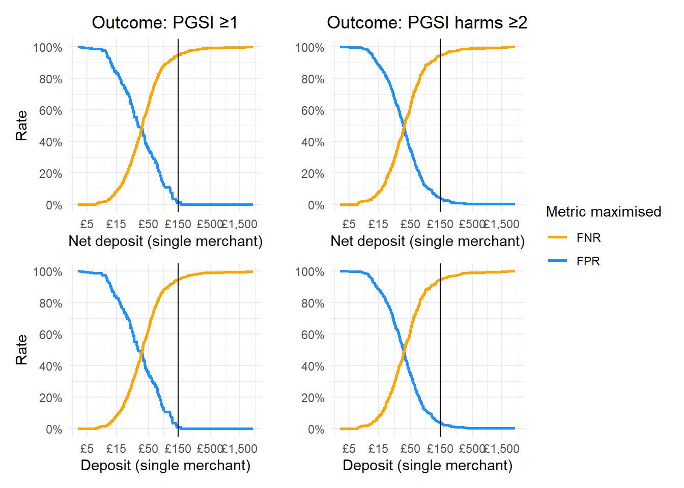
Now, we can use the cutpointr package to identify the optimal monthly deposit and net deposit values that differentiate at risk from not at risk consumers.
We will do this in several different ways, first maximising for the Youden Index, which balances sensitivity and specificity. We will maximise for sensitivity and then finally for specificity.
Make custom functions for threshold analyses
Let’s start by developing some custom functions to determine the optimal cut-off values alongside key performance metrics (e.g., sensitivity, specificity, accuracy) with CIs:
Show code
# Youden optimisation function: # Start by defining key variables/inputs for the cutpoint function:summarize_auc_results_youden <-function(data, predictor_var, outcome_var, pos_class, neg_class, subgroup, boot_runs =2000) { predictor_var <- rlang::ensym(predictor_var) outcome_var <- rlang::ensym(outcome_var)# Calculate Threshold value & AUC results for PGSI: youden_cutpoint <-cutpointr( data,!!predictor_var,!!outcome_var,pos_class = pos_class,neg_class = neg_class,method = maximize_boot_metric,metric = youden,direction =">=",boot_runs = boot_runs,na.rm =TRUE )# Calculate CI's for this: auc_cis <-boot_ci(youden_cutpoint, AUC, in_bag =TRUE, alpha =0.05) %>% dplyr::select(values) %>%t() %>%as_tibble() %>%mutate(across(everything(), ~round(as.numeric(.), 3))) %>%unite("95%CIs", V1, V2, sep =", ")# Isolate key results: auc_results <- youden_cutpoint %>% dplyr::select(predictor, optimal_cutpoint, AUC, sensitivity, specificity, acc) %>%mutate(Metric_maximised ="Youden")# Combine all results into a single summary table: auc_summary <-bind_cols(auc_results, auc_cis)return(auc_summary)}# Sensitivity optimisation function: # Start by defining key variables/inputs for the cutpoint function, This time noting that we are maximising sensitivity and constraining specificity to a minimum of 0.5:summarize_auc_results_max_sensitivity <-function(data, predictor_var, outcome_var, pos_class, neg_class, boot_runs =2000) {# Convert predictor_var and outcome_var to symbols for non-standard evaluation predictor_var <- rlang::ensym(predictor_var) outcome_var <- rlang::ensym(outcome_var)# Calculate Threshold value & AUC results sensitivity_cutpoint <-cutpointr( data,!!predictor_var,!!outcome_var,pos_class = pos_class,neg_class = neg_class,direction =">=",method = maximize_boot_metric, metric = sens_constrain,# constrain_metric = specificity, min_constrain =0.3,boot_runs = boot_runs,na.rm =TRUE )# Calculate Confidence Intervals auc_cis <-boot_ci(sensitivity_cutpoint, AUC, in_bag =TRUE, alpha =0.05) %>% dplyr::select(values) %>%t() %>%as_tibble() %>%mutate(across(everything(), ~round(as.numeric(.), 3))) %>%unite("95%CIs", V1, V2, sep =", ")# Isolate Key Results auc_results <- sensitivity_cutpoint %>% dplyr::select( predictor, optimal_cutpoint, AUC, sensitivity, specificity, acc ) %>%mutate(Metric_maximised ="Sensitivity")# Combine All Results auc_summary <-bind_cols(auc_results, auc_cis)return(auc_summary)}# Specificity optimisation function: # Start by defining key variables/inputs for the cutpoint function, This time noting that we are maximising Specificity and constraining Sensitivity to a minimum of 0.5:summarize_auc_results_max_specificity <-function(data, predictor_var, outcome_var, pos_class, neg_class, boot_runs =2000) {# Convert predictor_var and outcome_var to symbols for non-standard evaluation predictor_var <- rlang::ensym(predictor_var) outcome_var <- rlang::ensym(outcome_var)# Calculate Threshold value & AUC results spec_cutpoint <-cutpointr( data,!!predictor_var,!!outcome_var,pos_class = pos_class,neg_class = neg_class,method = maximize_boot_metric,metric = spec_constrain,# constrain_metric = sensitivity, min_constrain =0.3,direction =">=",boot_runs = boot_runs,na.rm =TRUE )# Calculate Confidence Intervals auc_cis <-boot_ci(spec_cutpoint, AUC, in_bag =TRUE, alpha =0.05) %>% dplyr::select(values) %>%t() %>%as_tibble() %>%mutate(across(everything(), ~round(as.numeric(.), 3))) %>%unite("95%CIs", V1, V2, sep =", ")# Isolate Key Results auc_results <- spec_cutpoint %>% dplyr::select( predictor, optimal_cutpoint, AUC, sensitivity, specificity, acc ) %>%mutate(Metric_maximised ="Specificity")# Combine All Results auc_summary <-bind_cols(auc_results, auc_cis)return(auc_summary)}
Let’s also create the same functions that allow us to split outcomes into subgroups by age:
One really important decision to make here is what value/variable we use to try and derive an optimal cut off for.
As a starting point, let’s think about using people’s average values across the year so the cut-offs will be based on a wider range of spending data than any single month.
This gives us two potential values to work with:
average_monthly_net_deposit_any_single_merchant (and the deposit only version: average_monthly_deposit_any_single_merchant)
average_monthly_net_deposit_all (and the deposit only version: average_monthly_deposit_any_single_merchant)
The first of these represents the average amount somebody spent with any single operator in any single month. So, if person A bet with Ladbrokes 2 months, spending £50 in February and £60 in April, and spent £20 with Betfair in Feb and £30 with Lottoland in May, their value for this variable would be £41.66: ((50+20)+60+30)/4. (this is for deposit only, not net deposit)
The second of these represents the average amount somebody spent across all operators in a single month (i.e., their total monthly gambling spend). Using Person A, this person’s value here would be: £53.3 (i.e., 50+20+60+30)/3).
I think it’s interesting to do both, but the first is most important as these checks will be done at the individual merchant level, at least for now.
Let’s first do the single operator values then total spend values.
Optimal single operator threshold values
Will start with net deposit then move to simple deposit values.
Net deposit - Simple PGSI grouping
Run functions for simple PGSI grouping, all participants:
Commented out code chunks
Note that all of the code that actually identifies optimal threshold values is commented out in the script as the bootstrapping process used takes a substantial amount of time. As such, the outcomes from these executions is loaded in later to save time, and also to avoid potentially producing variable outcomes with each run due to minor variations stemming from bootstrapping.
Now let’s see how performance changes if we change the predictor metric (i.e., the value along which we choose the threshold) to just simple deposit amount (again averaged over the months and operators/merchants to produce a monthly average deposit with any operator)
Run functions for simple PGSI grouping, all participants:
Start by combining everything and then saving them so we can load these outcomes in again later without having to rerun all of the bootstrapping:
Show code
# # Combine all outcomes from the any risk PGSI outcome (all ps and age split):# net_deposit_auc_combined_outcomes_any_risk<- bind_rows(Net_deposit_AUC_Youden_any_risk,# Net_deposit_AUC_Youden_any_risk_age_split,# Net_deposit_AUC_Sensitivity_any_risk,# Net_deposit_AUC_Sensitivity_any_risk_age_split,# Net_deposit_AUC_Specificity_any_risk,# Net_deposit_AUC_Specificity_any_risk_age_split) %>%# dplyr::select(-9)# # # Combine all outcomes from the PGSI harm outcome (all ps and age split):# net_deposit_auc_combined_outcomes_harm<- bind_rows(Net_deposit_AUC_Youden_harm,# Net_deposit_AUC_Youden_harm_age_split,# Net_deposit_AUC_Sensitivity_harm,# Net_deposit_AUC_Sensitivity_harm_age_split,# Net_deposit_AUC_Specificity_harm,# Net_deposit_AUC_Specificity_harm_age_split) %>%# dplyr::select(-9)# # # Join together the above to give us all outcomes relating to net deposit:# net_deposit_auc_combined_outcomes_all<- net_deposit_auc_combined_outcomes_any_risk %>%# bind_cols(net_deposit_auc_combined_outcomes_harm)# # # # # Combine all outcomes from the any risk PGSI outcome (all ps and age split):# Simple_deposit_auc_combined_outcomes_any_risk<- bind_rows(Simple_deposit_AUC_Youden_any_risk,# Simple_deposit_AUC_Youden_any_risk_age_split,# Simple_deposit_AUC_Sensitivity_any_risk,# Simple_deposit_AUC_Sensitivity_any_risk_age_split,# Simple_deposit_AUC_Specificity_any_risk,# Simple_deposit_AUC_Specificity_any_risk_age_split) %>%# dplyr::select(-9)# # # Combine all outcomes from the PGSI harm outcome (all ps and age split):# Simple_deposit_auc_combined_outcomes_harm<- bind_rows(Simple_deposit_AUC_Youden_harm,# Simple_deposit_AUC_Youden_harm_age_split,# Simple_deposit_AUC_Sensitivity_harm,# Simple_deposit_AUC_Sensitivity_harm_age_split,# Simple_deposit_AUC_Specificity_harm,# Simple_deposit_AUC_Specificity_harm_age_split) %>%# dplyr::select(-9)# # # Join together the above to give us all outcomes relating to simple deposit:# Simple_deposit_auc_combined_outcomes_all<- Simple_deposit_auc_combined_outcomes_any_risk %>%# bind_cols(Simple_deposit_auc_combined_outcomes_harm)# # # Save all of these outcomes:# write_csv(net_deposit_auc_combined_outcomes_all, "Data/net_deposit_auc_combined_outcomes_all_single_merchant")# write_csv(Simple_deposit_auc_combined_outcomes_all, "Data/Simple_deposit_auc_combined_outcomes_all_single_merchant")
Table optimal thresholds - single operator
Read in the saved datasets:
Actual dataset outcomes inserted from here
This is where we introduce the datasets produced by author DZ that result from running this exact same script on the actual dataset to produce a version of the data file created in the above chuck with the actual outcomes. So, the outcomes presented from here onwards should resemble those in our manuscript.
Show code
# Read in the actual datasets from David:net_deposit_auc_combined_outcomes_all_single_merchant <-read_csv("Data David/net_deposit_auc_combined_outcomes_all_single_merchant.csv")Simple_deposit_auc_combined_outcomes_all_single_merchant <-read_csv("Data David/Simple_deposit_auc_combined_outcomes_all_single_merchant.csv")
Make the table summarising the optimal thresholds for single operator spend:
Optimal threshold values with performance metrics for average monthly net deposit and deposit amounts (single merchant)
Subgroup
Metric Maximised
Outcome: PGSI ≥1
Outcome: PGSI harms ≥2
Balanced accuracy_h
Accuracy
Optimal threshold
AUC
95%CIs
Sensitivity
Specificity
Balanced accuracy
Accuracy
Optimal threshold
AUC
95%CIs
Sensitivity
Specificity
Net deposit amount
All participants
Youden
18.600
0.700
0.649, 0.748
0.564
0.738
0.6510
0.658
35.361
0.695
0.631, 0.752
0.492
0.859
0.6755
0.757
30+
Youden
17.366
0.698
0.636, 0.76
0.590
0.703
0.6465
0.658
35.707
0.711
0.631, 0.788
0.500
0.857
0.6785
0.774
Under 30
Youden
17.078
0.733
0.646, 0.82
0.551
0.852
0.7015
0.674
33.115
0.686
0.584, 0.788
0.480
0.841
0.6605
0.705
All participants
Sensitivity
4.744
0.700
0.65, 0.749
0.867
0.301
0.5840
0.561
6.136
0.695
0.63, 0.753
0.822
0.330
0.5760
0.467
30+
Sensitivity
6.023
0.698
0.633, 0.756
0.863
0.337
0.6000
0.548
7.541
0.711
0.628, 0.787
0.838
0.353
0.5955
0.466
Under 30
Sensitivity
2.557
0.733
0.641, 0.815
0.859
0.407
0.6330
0.674
4.900
0.686
0.575, 0.78
0.800
0.317
0.5585
0.500
All participants
Specificity
58.948
0.700
0.651, 0.751
0.308
0.930
0.6190
0.644
96.254
0.695
0.635, 0.757
0.288
0.948
0.6180
0.764
30+
Specificity
57.273
0.698
0.637, 0.758
0.316
0.914
0.6150
0.675
121.558
0.711
0.632, 0.784
0.279
0.960
0.6195
0.801
Under 30
Specificity
51.658
0.733
0.648, 0.82
0.295
0.963
0.6290
0.568
86.258
0.686
0.586, 0.78
0.280
0.951
0.6155
0.697
Deposit amount
All participants
Youden
16.082
0.706
0.656, 0.754
0.569
0.760
0.6645
0.672
25.121
0.705
0.643, 0.762
0.517
0.817
0.6670
0.733
30+
Youden
15.042
0.707
0.642, 0.77
0.624
0.703
0.6635
0.671
29.262
0.725
0.646, 0.801
0.529
0.844
0.6865
0.771
Under 30
Youden
15.234
0.738
0.652, 0.822
0.564
0.852
0.7080
0.682
20.156
0.692
0.588, 0.791
0.540
0.793
0.6665
0.697
All participants
Sensitivity
3.566
0.706
0.657, 0.753
0.882
0.328
0.6050
0.583
5.873
0.705
0.642, 0.762
0.822
0.363
0.5925
0.491
30+
Sensitivity
5.332
0.707
0.643, 0.765
0.838
0.354
0.5960
0.548
6.679
0.725
0.644, 0.797
0.853
0.375
0.6140
0.486
Under 30
Sensitivity
2.543
0.738
0.648, 0.818
0.859
0.463
0.6610
0.697
4.008
0.692
0.585, 0.787
0.820
0.354
0.5870
0.530
All participants
Specificity
39.843
0.706
0.655, 0.759
0.292
0.908
0.6000
0.625
78.092
0.705
0.646, 0.764
0.297
0.954
0.6255
0.771
30+
Specificity
43.602
0.707
0.646, 0.765
0.308
0.897
0.6025
0.661
89.572
0.725
0.648, 0.794
0.294
0.964
0.6290
0.808
Under 30
Specificity
32.583
0.738
0.652, 0.823
0.321
0.944
0.6325
0.576
62.322
0.692
0.594, 0.783
0.300
0.939
0.6195
0.697
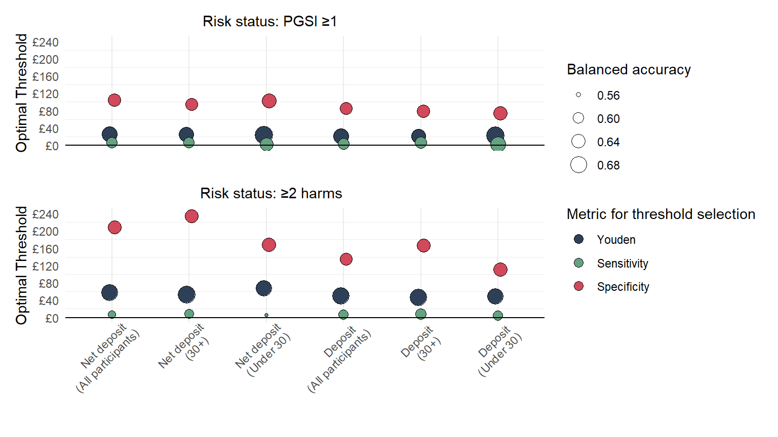
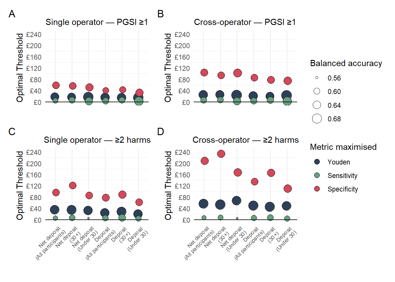
Plot optimal thresholds - single operator
There is a huge amount of information in the above table (we extract parts of it and separate it into separate tables in the manuscript)… let’s see if we can make some kind of plot that summarises the key takeaways:
Show code
optimal_cut_point_plot_data_single_operator<-bind_rows(net_deposit_auc_combined_outcomes_all_single_merchant, Simple_deposit_auc_combined_outcomes_all_single_merchant) %>%mutate(across(where(is.numeric), ~round(., 3)),Subgroup =case_when(is.na(`subgroup...9`) ~"All participants",TRUE~`subgroup...9`) ) %>%# Create balanced accuracy vars:mutate('Balanced accuracy'= (`sensitivity...4`+`specificity...5`)/2,'Balanced accuracy_h'= (`sensitivity...13`+`specificity...14`)/2) %>%# Select relevant vars: dplyr::select(Variable ='predictor...1', Subgroup,'Metric Maximised'='Metric_maximised...7','Optimal threshold'='optimal_cutpoint...2',Sensitivity ='sensitivity...4',Specificity ='specificity...5','Balanced accuracy','Optimal threshold_h'='optimal_cutpoint...11',Sensitivity_h ='sensitivity...13',Specificity_h ='specificity...14','Balanced accuracy_h' ) # Set factor levels to control orderoptimal_cut_point_plot_data_single_operator <- optimal_cut_point_plot_data_single_operator %>%mutate(Subgroup =factor(Subgroup, levels =c("All participants", "30+", "Under 30")),Metric =factor(`Metric Maximised`, levels =c("Youden", "Sensitivity", "Specificity")),Variable_Subgroup =interaction(Variable, Subgroup, sep =" - ", lex.order =TRUE) )# Create a grouped x-axis factor that preserves desired order of Subgroup within each Variableoptimal_cut_point_plot_data_single_operator <- optimal_cut_point_plot_data_single_operator %>%mutate(Subgroup =factor(Subgroup, levels =c("All participants", "30+", "Under 30")),Metric =factor(`Metric Maximised`, levels =c("Youden", "Sensitivity", "Specificity")),Variable_Subgroup =factor(paste(case_when( Variable =="average_monthly_deposit_any_single_merchant"~"Deposit", Variable =="average_monthly_net_deposit_any_single_merchant"~"Net deposit" ), Subgroup,sep =" - " ), levels =c("Net deposit - All participants","Net deposit - 30+","Net deposit - Under 30","Deposit - All participants","Deposit - 30+","Deposit - Under 30" )) ) x_labels <-c("Net deposit\n(All participants)","Net deposit\n(30+)","Net deposit\n(Under 30)","Deposit\n(All participants)","Deposit\n(30+)","Deposit\n(Under 30)")# I need the scale for the legends to be consistent across the two parts, so find the range of values:size_vals <-c(optimal_cut_point_plot_data_single_operator$`Balanced accuracy`, optimal_cut_point_plot_data_single_operator$`Balanced accuracy_h`)scale_limits <-range(size_vals, na.rm =TRUE)common_size_scale <-scale_size_continuous(name ="Balanced accuracy",limits = scale_limits,range =c(1, 6) )# Create plot for predicting 1+ on PGSI:threshold_plot_single_operator_simple_pgsi<-ggplot(optimal_cut_point_plot_data_single_operator, aes(x = Variable_Subgroup, y =`Optimal threshold`, color = Metric, size =`Balanced accuracy`)) +geom_point(shape =21, stroke =0.5, color ="black", aes(fill = Metric, size =`Balanced accuracy`), position =position_dodge(width =0)) +scale_fill_manual(values =c("Youden"="#2e4057", "Sensitivity"="#66a182", "Specificity"="#d1495b")) +scale_x_discrete(labels = x_labels) +scale_y_continuous(limits =c(0, 122), breaks =seq(0, 120, 30),labels = scales::label_currency(prefix ="£",big.mark =",", accuracy =1)) +labs(x ="",y ="Optimal Threshold",fill ="Metric for threshold selection",size ="Balanced accuracy",title ="Risk status: PGSI ≥1" ) +theme_minimal() +geom_hline(yintercept =0, size = .5, color ="black") +theme(axis.text.x =element_blank(),text=element_text(family="Poppins"),plot.title =element_text(hjust =0.4, size =11),# axis.text.x = element_text(angle = 45, hjust = 0.8),panel.grid.major.y =element_blank() ) + common_size_scale +guides(fill =guide_legend(override.aes =list(size =3)),size =guide_legend() )# Create plot for predicting 2+ harms on PGSI:threshold_plot_single_operator_2plus_harms<-ggplot(optimal_cut_point_plot_data_single_operator, aes(x = Variable_Subgroup, y =`Optimal threshold_h`, color = Metric, size =`Balanced accuracy_h`)) +geom_point(shape =21, stroke =0.5, color ="black", aes(fill = Metric, size =`Balanced accuracy_h`), position =position_dodge(width =0)) +scale_fill_manual(values =c("Youden"="#2e4057", "Sensitivity"="#66a182", "Specificity"="#d1495b")) +scale_x_discrete(labels = x_labels) +scale_y_continuous(limits =c(0, 128), breaks =seq(0, 120, 30),labels = scales::label_currency(prefix ="£", big.mark =",", accuracy =1)) +labs(x ="",y ="Optimal Threshold",fill ="Metric for thresholds selection",size ="Balanced accuracy",title ="Risk status: ≥2 harms" ) +theme_minimal() +geom_hline(yintercept =0, size = .5, color ="black") + common_size_scale +theme(legend.position ="none",text=element_text(family="Poppins"),axis.text.x =element_text(angle =45, hjust =0.8),plot.title =element_text(hjust =0.4, size =11),panel.grid.major.y =element_blank() ) theshold_plot_single_operator_final <- threshold_plot_single_operator_simple_pgsi/threshold_plot_single_operator_2plus_harms +plot_layout(guides ='collect')ggsave(filename ="Figures/theshold_plot_single_operator_final.pdf",plot = theshold_plot_single_operator_final,width =7,height =5,units ="in",dpi =600)
Summary stats
Below we produce some basic summary outcomes for AUC values.
What’s the average AUC for net-deposit values when risk status is defined by PGSI scores of 1+?
# # Combine all outcomes from the any risk PGSI outcome (all ps and age split):# net_deposit_auc_combined_outcomes_any_risk<- bind_rows(Net_deposit_AUC_Youden_any_risk,# Net_deposit_AUC_Youden_any_risk_age_split,# Net_deposit_AUC_Sensitivity_any_risk,# Net_deposit_AUC_Sensitivity_any_risk_age_split,# Net_deposit_AUC_Specificity_any_risk,# Net_deposit_AUC_Specificity_any_risk_age_split) %>%# dplyr::select(-9)# # # Combine all outcomes from the PGSI harm outcome (all ps and age split):# net_deposit_auc_combined_outcomes_harm<- bind_rows(Net_deposit_AUC_Youden_harm,# Net_deposit_AUC_Youden_harm_age_split,# Net_deposit_AUC_Sensitivity_harm,# Net_deposit_AUC_Sensitivity_harm_age_split,# Net_deposit_AUC_Specificity_harm,# Net_deposit_AUC_Specificity_harm_age_split) %>%# dplyr::select(-9)# # # Join together the above to give us all outcomes relating to net deposit:# net_deposit_auc_combined_outcomes_all<- net_deposit_auc_combined_outcomes_any_risk %>%# bind_cols(net_deposit_auc_combined_outcomes_harm) # # # # # Combine all outcomes from the any risk PGSI outcome (all ps and age split):# Simple_deposit_auc_combined_outcomes_any_risk<- bind_rows(Simple_deposit_AUC_Youden_any_risk,# Simple_deposit_AUC_Youden_any_risk_age_split,# Simple_deposit_AUC_Sensitivity_any_risk,# Simple_deposit_AUC_Sensitivity_any_risk_age_split,# Simple_deposit_AUC_Specificity_any_risk,# Simple_deposit_AUC_Specificity_any_risk_age_split) %>%# dplyr::select(-9)# # # Combine all outcomes from the PGSI harm outcome (all ps and age split):# Simple_deposit_auc_combined_outcomes_harm<- bind_rows(Simple_deposit_AUC_Youden_harm,# Simple_deposit_AUC_Youden_harm_age_split,# Simple_deposit_AUC_Sensitivity_harm,# Simple_deposit_AUC_Sensitivity_harm_age_split,# Simple_deposit_AUC_Specificity_harm,# Simple_deposit_AUC_Specificity_harm_age_split) %>%# dplyr::select(-9)# # # Join together the above to give us all outcomes relating to simple deposit:# Simple_deposit_auc_combined_outcomes_all<- Simple_deposit_auc_combined_outcomes_any_risk %>%# bind_cols(Simple_deposit_auc_combined_outcomes_harm) # # # Save all of these outcomes:# write_csv(net_deposit_auc_combined_outcomes_all, "Data/net_deposit_auc_combined_outcomes_all_combined_merchants")# write_csv(Simple_deposit_auc_combined_outcomes_all, "Data/Simple_deposit_auc_combined_outcomes_all_combined_merchants")
Read in the saved datasets and make our table, again noting we are loading in datasets produced by author DZ here:
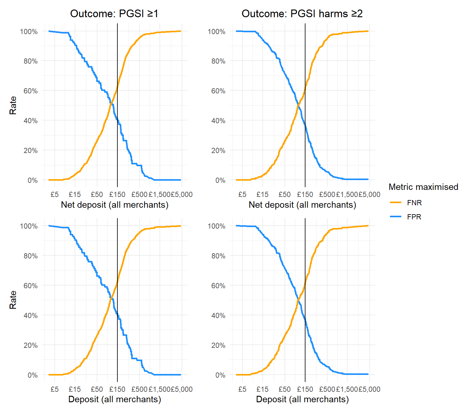
Now compute the error rates for both outcomes and both predictors (noting again that this is not based on the actual data, and is based on the simulated dataset):
Show code
# Calculate trade-offs for net deposit with PSGI >0 as the outcometradeoff_data_net_deposit_any_risk <-calculate_tradeoff(data = combined_data_monthly_averages_all_merchants,predictor_var = average_monthly_net_deposit_all,outcome_var = PGSI_GROUPING_SIMPLE,pos_class ="At risk",neg_class ="No risk")# And plot:net_deposit_any_risk_graph<-ggplot(tradeoff_data_net_deposit_any_risk, aes(x = Threshold)) +geom_line(aes(y = FPR, color ="FPR"), size =1) +geom_line(aes(y = FNR, color ="FNR"), size =1) +labs(title ="Outcome: PGSI ≥1",x ="Net deposit (all merchants)",y ="Rate",color ="Metric maximised" ) +scale_color_manual(values =c("FPR"="dodgerblue", "FNR"="orange")) +scale_x_continuous(trans="log10",labels =function(x) paste0("£", scales::comma(x)),breaks =c(0,5,15,50,150,500,1500,5000)) +scale_y_continuous(labels = scales::percent_format(scale =100), breaks =seq(0, 1, by =0.2)) +geom_vline(xintercept =c(150), color ="black") +theme_minimal() +theme(text=element_text(family="Poppins"),plot.title =element_text(hjust =0.5))# Calculate trade-offs for net deposit with PSI harm as the outcometradeoff_data_net_deposit_harm <-calculate_tradeoff(data = combined_data_monthly_averages_all_merchants,predictor_var = average_monthly_net_deposit_all,outcome_var = PGSI_GROUPING_HARM,pos_class ="Harm",neg_class ="No harm")# And plot:net_deposit_harm_graph<-ggplot(tradeoff_data_net_deposit_harm, aes(x = Threshold)) +geom_line(aes(y = FPR, color ="FPR"), size =1) +geom_line(aes(y = FNR, color ="FNR"), size =1) +labs(title ="Outcome: PGSI harms ≥2",x ="Net deposit (all merchants)",y ="",color ="Metric maximised" ) +theme_minimal() +scale_color_manual(values =c("FPR"="dodgerblue", "FNR"="orange")) +scale_x_continuous(trans="log10",labels =function(x) paste0("£", scales::comma(x)),breaks =c(0,5,15,50,150,500,1500,5000)) +scale_y_continuous(labels = scales::percent_format(scale =100), breaks =seq(0, 1, by =0.2)) +geom_vline(xintercept =c(150), color ="black") +theme_minimal() +theme(text=element_text(family="Poppins"),plot.title =element_text(hjust =0.5) )# Calculate trade-offs for simple deposit with PSGI >0 as the outcometradeoff_data_simple_deposit_any_risk <-calculate_tradeoff(data = combined_data_monthly_averages_all_merchants,predictor_var = average_monthly_deposit_all,outcome_var = PGSI_GROUPING_SIMPLE,pos_class ="At risk",neg_class ="No risk")# And plot:simple_deposit_any_risk_graph<-ggplot(tradeoff_data_simple_deposit_any_risk, aes(x = Threshold)) +geom_line(aes(y = FPR, color ="FPR"), size =1) +geom_line(aes(y = FNR, color ="FNR"), size =1) +labs(x ="Deposit (all merchants)",y ="Rate",color ="Metric maximised" ) +theme_minimal() +scale_color_manual(values =c("FPR"="dodgerblue", "FNR"="orange")) +scale_x_continuous(trans="log10",labels =function(x) paste0("£", scales::comma(x)),breaks =c(0,5,15,50,150,500,1500,5000)) +scale_y_continuous(labels = scales::percent_format(scale =100), breaks =seq(0, 1, by =0.2)) +geom_vline(xintercept =c(150), color ="black") +theme_minimal() +theme(text=element_text(family="Poppins"))# Calculate trade-offs for simple deposit with PSI harm as the outcometradeoff_data_simple_deposit_harm <-calculate_tradeoff(data = combined_data_monthly_averages_all_merchants,predictor_var = average_monthly_deposit_all,outcome_var = PGSI_GROUPING_HARM,pos_class ="Harm",neg_class ="No harm")# And plot:simple_deposit_harm_graph<-ggplot(tradeoff_data_simple_deposit_harm, aes(x = Threshold)) +geom_line(aes(y = FPR, color ="FPR"), size =1) +geom_line(aes(y = FNR, color ="FNR"), size =1) +labs(x ="Deposit (all merchants)",y ="",color ="Metric maximised" ) +theme_minimal() +scale_color_manual(values =c("FPR"="dodgerblue", "FNR"="orange")) +scale_x_continuous(trans="log10",labels =function(x) paste0("£", scales::comma(x)),breaks =c(0,5,15,50,150,500,1500,5000)) +scale_y_continuous(labels = scales::percent_format(scale =100), breaks =seq(0, 1, by =0.2)) +geom_vline(xintercept =c(150), color ="black") +theme_minimal() +theme(text=element_text(family="Poppins"))fp_fn_trade_off_plot_all_operators <- (net_deposit_any_risk_graph + net_deposit_harm_graph)/(simple_deposit_any_risk_graph + simple_deposit_harm_graph) +plot_layout(guides ='collect')fp_fn_trade_off_plot_all_operators
Asses the internal reliability of PGSI scores to report in our manuscript:
Show code
PGSI_scores<- survey_data_processed %>% dplyr::select(starts_with("PGSI"),-PGSI_TOTAL)cronbach.alpha(PGSI_scores, standardized =FALSE, CI =FALSE, probs =c(0.025, 0.975), B =1000, na.rm =FALSE)
Cronbach's alpha for the 'PGSI_scores' data-set

Items: 13
Sample units: 651
alpha: 0.74
Reproducibility of this analysis
Package stability
To ensure that every time this script runs it will use the same versions of the packages used during the script development, all packages are loaded using the groundhog.library() function from the groundhog package.
Rendering & publishing
This document is rendered in HTML format and published online using Quarto Pub. Use the following command in the terminal to publish:
quarto publish quarto-pub affordability_checks_analysis.qmd
Session details
Expand for session information
Warning in system2("quarto", "-V", stdout = TRUE, env = paste0("TMPDIR=", :
running command '"quarto"
TMPDIR=C:/Users/rhei4496/AppData/Local/Temp/Rtmpyc7Xti/file81a87c3a49 -V' had
status 1